AMReX – a block-structured Adaptive Mesh Refinement (AMR) framework
At a Glance
Questions                 |Objectives                           |Key Points
--------------------------|----------- -------------------------|--------------------------
How do I start to use     | Understand easy set-up              | It's not hard to get started
AMReX?                    |                                     |
                          |                                     |
How do I 'turn on' AMR?   | Understand minimum specs for AMR    | When the algorithm is correctly designed
                          |                                     | and implemented, AMR 'just works'
                          |                                     |
How do I visualize AMR    | Use Visit for AMR results           | Visualization tools exist for AMR data.
results?
Example: Single-Level Heat Equation
The Equation and the Discretization
First lets revisit the heat equation problem.
This algorithm should look familiar to you – in each time step we call the following two Fortran routines:
  ! x-fluxes
  do    j = lo(2), hi(2)
     do i = lo(1), hi(1)+1
        fluxx(i,j) = ( phi(i,j) - phi(i-1,j) ) / dx(1)
     end do
  end do

  ! y-fluxes
  do    j = lo(2), hi(2)+1
     do i = lo(1), hi(1)
        fluxy(i,j) = ( phi(i,j) - phi(i,j-1) ) / dx(2)
     end do
  end do
and
  do    j = lo(2), hi(2)
     do i = lo(1), hi(1)

        phinew(i,j) = phiold(i,j) &
             + dtdx(1) * (fluxx(i+1,j  ) - fluxx(i,j)) &
             + dtdx(2) * (fluxy(i  ,j+1) - fluxy(i,j))

     end do
  end do
The other parts of the algorithm – that, in particular, involve MPI communication, are handled in the C++:
MultiFab::Copy(phi_old, phi_new, 0, 0, 1, 0);
and
old_phi.FillBoundary(geom.periodicity());
See if it makes sense what order all of these are called in.
Running the Problem
Note: To run this part of the lesson
cd handson/amrex/AMReX_diffusion
In this directory you’ll see
main2d.gnu.MPI.ex -- the executable
inputs_2d -- the inputs file
fextract -- an executable that extracts a 1-d slice from 2-d or 3-d data
extract_slice -- a simple script that calls fextract on each of our plotfiles
plot_phi -- a simple gnuplot script to read and animate the 1-d slices
The inputs file currently has
nsteps = 20000
n_cell = 256 256
max_grid_size = 128
plot_int = 1000
is_periodic = 1 0
The grid is a cube consisting of 256 x 256 cells, consisting of 4 subgrids each of size 128x128 cells. The problem is periodic in the x-direction and not in the y-direction. This problem happens to be set-up to have homogeneous Neumann boundary conditions when not periodic.
Let’s try running this 2-d problem
./main2d.gnu.MPI.ex inputs_2d
Then let’s extract 1-d slices from the plotfiles and animate them
source extract_slice
gnuplot plot_phi
This should make an animated gif like the one you see here.
 |
If you’d like to see the 2-d solution, use Visit to open up a plotfile.
Select ``File'' then ``Open file ...'',
then select the Header file associated the the plotfile of interest (e.g., _plt00000/Header_
Here are instructions (from the Users Guide) for making a simple plot:

To view the data, select ``Add'' then ``Pseudocolor'' then ``phi'' then ``Draw''.

To view the grid structure (not particularly interesting yet, but when we add AMR it will be), select
``subset'' then ``levels''.  Then double-click the text ``Subset - levels'',
enable the ``Wireframe'' option, select ``Apply'', select ``Dismiss'', and then select ``Draw''.

To save the image, select ``File'' then ``Set save options'', then customize the image format
to your liking, then click ``Save''.
Your images should look similar to those below.
| Time Step 0 | Time Step 10000 |
|---|---|
 |
 |
What does this do in parallel
Let’s now try
mpiexec -n 1 ./main2d.gnu.MPI.ex inputs_2d plot_int=-1 max_step= 1000  | grep "Run time"
mpiexec -n 2 ./main2d.gnu.MPI.ex inputs_2d plot_int=-1 max_step= 1000  | grep "Run time"
mpiexec -n 4 ./main2d.gnu.MPI.ex inputs_2d plot_int=-1 max_step= 1000  | grep "Run time"
and see how the timings compare.
Questions to think about:
Why did we set plot_int = -1 in the command line?
If this didn’t scale perfectly, why not?
Example: Multi-Level Advection
The Equation and the Discretization
Now let’s consider scalar advection with a specified time-dependent velocity field. In this example we’ll be using AMR.
This algorithm should also look familiar to you – in each time step we construct fluxes and use them to update the solution.
  ! Do a conservative update
  do    j = lo(2),hi(2)
     do i = lo(1),hi(1)
        uout(i,j) = uin(i,j) + &
             ( (flxx(i,j) - flxx(i+1,j)) * dtdx(1) &
             + (flxy(i,j) - flxy(i,j+1)) * dtdx(2) )
     enddo
  enddo
Here the construction of the fluxes is a little more complicated, and because we are going to use AMR, we must save the fluxes at each level so that we can use them in a refluxing operation. The subcycling in time algorithm, which we haven’t really had time to talk about, looks like
    if (lev < finest_level)
    {
        // recursive call for next-finer level
        for (int i = 1; i <= nsubsteps[lev+1]; ++i)
        {
            timeStep(lev+1, time+(i-1)*dt[lev+1], i);
        }

        if (do_reflux)
        {
            // update lev based on coarse-fine flux mismatch
            flux_reg[lev+1]->Reflux(*phi_new[lev], 1.0, 0, 0, phi_new[lev]->nComp(), geom[lev]);
        }

        AverageDownTo(lev); // average lev+1 down to lev
    }
Running the Problem
Note: To run this part of the lesson
cd handson/amrex/AMReX_advection
In this directory you’ll see
main2d.gnu.MPI.ex -- the executable
inputs -- the inputs file
The inputs file currently has
max_step = 120
amr.n_cell = 64 64
amr.max_grid_size = 32
amr.plot_int = 10
The grid here is a cube consisting of 64 x 64 cells, consisting of 4 subgrids each of size 32x32 cells. The problem is periodic in the x-direction and not in the y-direction. This problem happens to be set-up to have homogeneous Neumann boundary conditions when not periodic.
Let’s try running this 2-d problem with no refinement
./main2d.gnu.MPI.ex inputs amr.max_level=0
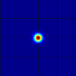
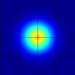
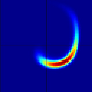
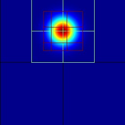
To see the 2-d solution, use Visit to look at plt00000 and plt00060, for example. You should see something like this (though these pictures are made using a different visualization program.)
| Time Step 0 | Time Step 60 |
|---|---|
 |
 |
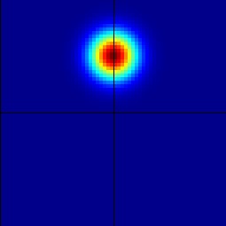
Now let’s turn on AMR.
Let’s now run with
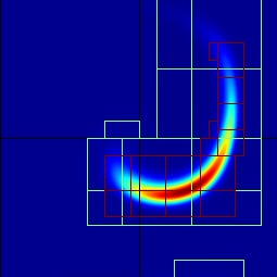
./main2d.gnu.MPI.ex inputs amr.max_level=2
and again visualize the results.
| Time Step 0 | Time Step 60 |
|---|---|
 |
 |
Further Reading
Learn more about AMReX here and take a look at the Users Guide in Docs.