Hand Coded 1D Heat Equation

At a Glance

Questions                 |Objectives                           |Key Points
--------------------------|-------------------------------------|-------------------------------------
What is a numerical alg.? |Understand performance metrics       |HPC numerical software involves complex
                          |                                     |algorithms and data structures.
                          |                                     |
What is discretization?   |Understand algorithmic trade-offs    |Robust software requires significant
                          |                                     |software quality engineering (SQE).
                          |                                     |
What is stability?        |Understand value of software packages|Numerical packages simplify app dev.,
                          |                                     |offer efficient & scalable performance,
                          |                                     |and enable app-specific customization.

Note: To run the application in this lesson

cd handson/handheat

Note: After each run, there are sometimes Q&A sections. To reveal answers, triple-click in the box below the answer.

Question:? (triple-click box to reveal answer)

Answer

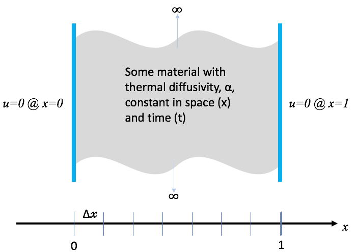
A Real-World Heat Problem

In this lesson, we demonstrate the design and use of a hand-coded (e.g., does not use any software packages) C-language application to model heat conduction through a wall as pictured here …

where the initial condition is two spikes of heat at two, non-symmetrically positioned points in x.

Governing Equations

In general, heat conduction is governed by the partial differential (PDE)…

$\frac{\partial u}{\partial t} - \nabla \cdot \alpha \nabla u = 0$

(1)

where u is the temperature within the wall at spatial positions, x, and times, t, $\alpha$ is the thermal diffusivity of the material(s) comprising the wall. This equation is known as the Diffusion Equation and also the Heat Equation.

Simplifying Assumptions

To make the problem tractable for this lesson, we make some simplifying assumptions…

The thermal diffusivity, $\alpha$ , is constant for all space and time.
The only heat source is from the initial and/or boundary conditions.
We will deal only with the one dimensional problem in Cartesian coordinates.

In this case, the PDE we need to develop an application to solve simplifies to…

$\frac{\partial u}{\partial t} = \alpha \frac{\partial^2 u}{\partial x^2}$

(2)

Scienitifc Inquiries

We want the application we develop to be useful in various scientific inquries such as…

Will the temperature at x=A exceed a given value?
How does the maximum temperature in the wall change with time?
At what time will temperature fluctuations of frequency, f , fall below a threshold?

To answer questions such as these, the application needs to be designed so that it can properly model time varying or transient behavior of heat conduction and not just thermal equilibrium.

Some Key Design Choices

Do we care only about the steady state or do we also care about the time varying or transient solution?
The PDE in equation 2 is a continuous equation in two independent variables x and t. How will we discretize the PDE so that we can calculate its solution in a computer program?
How do we develop the software so that extending it to solve more complex problems later is easy?

The Application Source Code

FTCS Discretization

Consider discretizing, independently, the left- and right-hand sides of equation 2. For the left-hand side, we can approximate the first derivative of u with respect to time, t, by the equation…

$\frac{\partial u}{\partial t} \Bigr|_{t_{k+1}} \approx \frac{u_i^{k+1}-u_i^k}{\Delta t}$

(3)

We can approximate the right-hand side of equation 2 with the second derivative of u with respect to space, x, by the equation…

$\alpha \frac{\partial^2 u}{\partial x^2}\Bigr|_{x_i} \approx \alpha \frac{u_{i-1}^k-2u_i^k+u_{i+1}^k}{\Delta x^2}$

(4)

Setting equations 3 and 4 equal to each other and re-arranging terms, we arrive at the following update scheme for producing the temperatures at the next time, k+1, from temperatures at the current time, k, as

$u_i^{k+1} = ru_{i+1}^k+(1-2r)u_i^k+ru_{i-1}^k$

(5)

where $r=\alpha\frac{\Delta t}{\Delta x^2}$

Is there anything in the discrete form of the PDE that looks like a mesh?

In the process of discretizing the PDE, we have defined a fixed spacing in x and a fixed spacing in t. This is essentially a uniform mesh. Later lessons here address more sophisticated discretizations in space and in time which depart from these all too inflexible fixed spacings.

Note that this equation now defines the solution at spatial position i and time k+1 in terms of values of u at time k . This is an explicit numerical method. Explicit methods have some nice properties:

They are easy to implement.
They typically require minimal memory.
They are easy to parallelize.

The code to implement this numerical method is shown below.

static void
solution_update_ftcs(int n,
    double *curr, double const *last,
    double alpha, double dx, double dt,
    double bc_0, double bc_1)
{
    double const r = alpha * dt / (dx * dx);

    /* Impose boundary conditions for solution indices i==0 and i==n-1 */
    curr[0  ] = bc_0;
    curr[n-1] = bc_1;

    /* Update the solution using FTCS algorithm */
    for (int i = 1; i < n-1; i++)
        curr[i] = r*last[i+1] + (1-2*r)*last[i] + r*last[i-1];
}

The FTCS update method is implemented around line 360 in the example application, heat.c.

Compiling heat.c

gcc -O3 -DHAVE_FEENABLEEXCEPT heat.c -o heat -lm

Getting Help

At any point, you can get help regarding various options the application supports like so…

$ ./heat --help
Usage:
    ./heat <arg>=<value> <arg>=<value>...
        prec=double                     precision half|float|double|quad (char*)
        alpha=0.2                          material thermal diffusivity (double)
        dx=0.1                                  x-incriment (1/dx->int) (double)
        dt=0.004                                            t-incriment (double)
        maxt=2                           max. time to run simulation to (double)
        bc0=0                                          bc @ x=0: u(0,t) (double)
        bc1=1                                          bc @ x=1: u(1,t) (double)
        ic=const(1)                                     ic @ t=0: u(x,0) (char*)
        alg=ftcs                          algorithm ftcs|upwind15|crankn (char*)
        savi=0                               save every i-th solution step (int)
        save=0                          save error in every saved solution (int)
        outi=100                  output progress every i-th solution step (int)
        noout=0                                   disable all file outputs (int)
Examples...
    ./heat dx=0.01 dt=0.0002 alg=ftcs
    ./heat dx=0.1 bc0=5 bc1=10 ic="spikes(5,5)"

Run 1

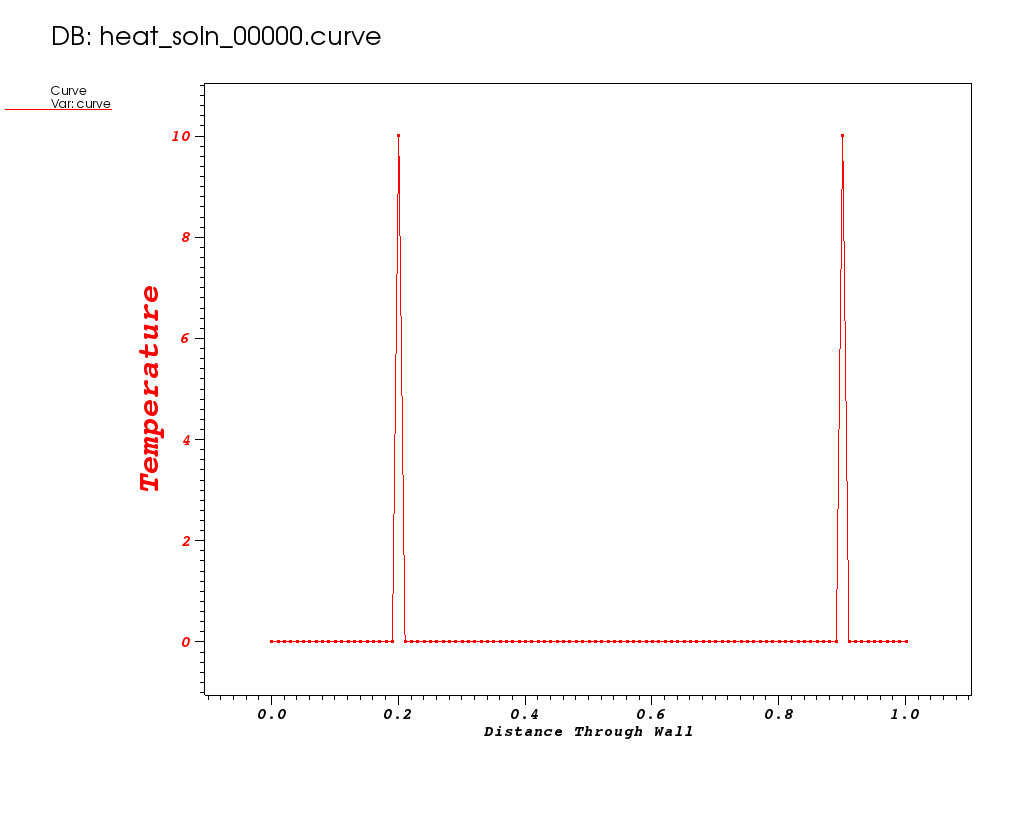
Let’s use this method to model the time evolution of heat from the initial condition pictured here…

to a maximum time of 2 seconds.

make basic_spikes
./heat bc1=0 ic="spikes(10,2,10,9)" savi=25
    prec=double
    alpha=0.2
    dx=0.1
    dt=0.004
    maxt=2
    bc0=0
    bc1=0
    ic=spikes(10,2,10,9)
    alg=ftcs
    savi=25
    save=0
    outi=100
    noout=0
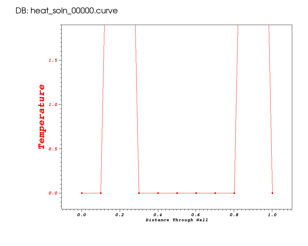
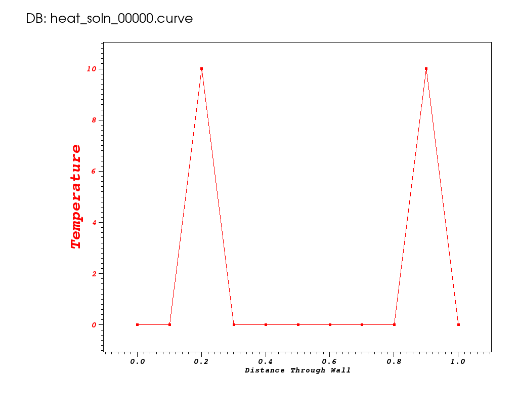
Timestep 0000: last change l2=7.04
Timestep 0100: last change l2=0.00021002
Timestep 0200: last change l2=4.25035e-05
Timestep 0300: last change l2=8.81977e-06
Timestep 0400: last change l2=1.83059e-06
Timestep 0500: last change l2=3.8597e-07
Integer ops        = 3285657
Floating point ops = 50310
Memory used        = 194 bytes

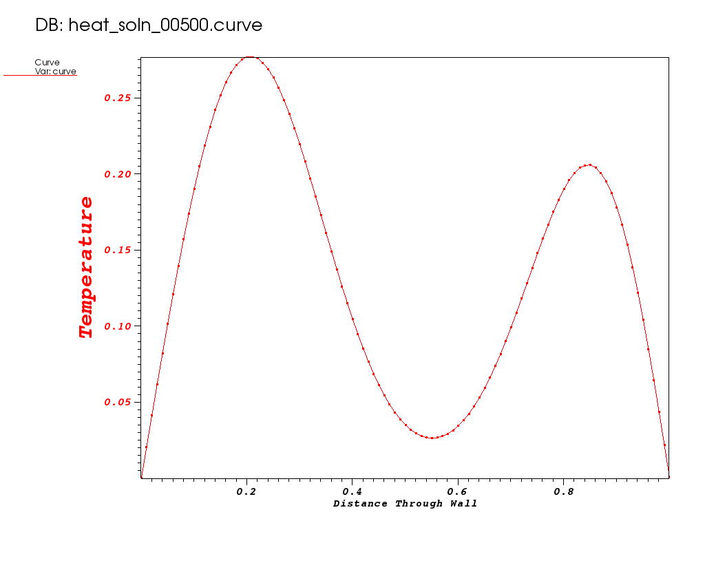
Take note of number of flops and memory used so we can compare these metrics to other runs later. The solution is plotted below for some key timesteps.

Time 0	Time 0.1	Time 0.5

Are the results correct? How would we assess that?

Writing custom code often also requires additional work to vett the results obtained, whereas relying upon mature community adopted software packages often means results those packages produce have already been well vetted in many regimes of interest.

Will I get the same results when using other computing platforms and compilers? Is the code we’ve written portable enough even to support that?

Maybe. In this overly simplified 500-line example program, it's conceivable that we could get numerically identical results when using numerous different platforms and compilers. However, imagine trying to do that with applications requiring highly sophisticated numerical algorithms and involving hundreds of thousands of lines of code, running on high-performance machines where we must also explicitly consider parallelism and architectural heterogeneity. A key advantage of using mature numerical packages is that many of these details have already been addressed by people who have deep expertise with high-performance algorithms and software.

Run 2

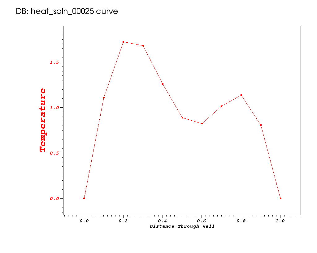
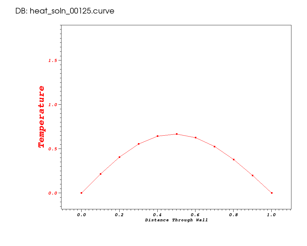
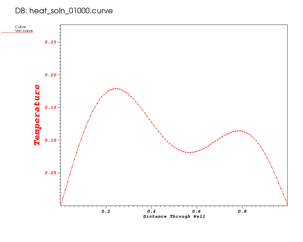
Now, suppose the science questions we need to answer require that we do a better job resolving the transient local temperature minimum that occurs at early time around x=0.6, as shown below from time 0.1 seconds.

To do this, we can try to increase the spatial resolution. Lets try dx=0.01.

[mcmiller@cooleylogin2 ~/tmp]$ make hr_spikes
./heat dx=0.01 bc1=0 ic="spikes(10,20,10,90)" savi=10
    prec=double
    alpha=0.2
    dx=0.01
    dt=0.004
    maxt=2
    bc0=0
    bc1=0
    ic=spikes(10,20,10,90)
    alg=ftcs
    savi=10
    save=0
    outi=100
    noout=0
Timestep 0000: last change l2=76800
Timestep 0100: last change l2=1.38688e+302
/bin/sh: line 8: 835744 Floating point exception
Integer ops        = 4392943
Floating point ops = 455350
Memory used        = 1636 bytes

Plots from some early times in the run are shown below…

Time 0	Time 0.01	Time 0.02

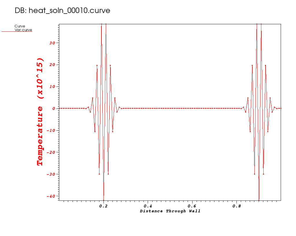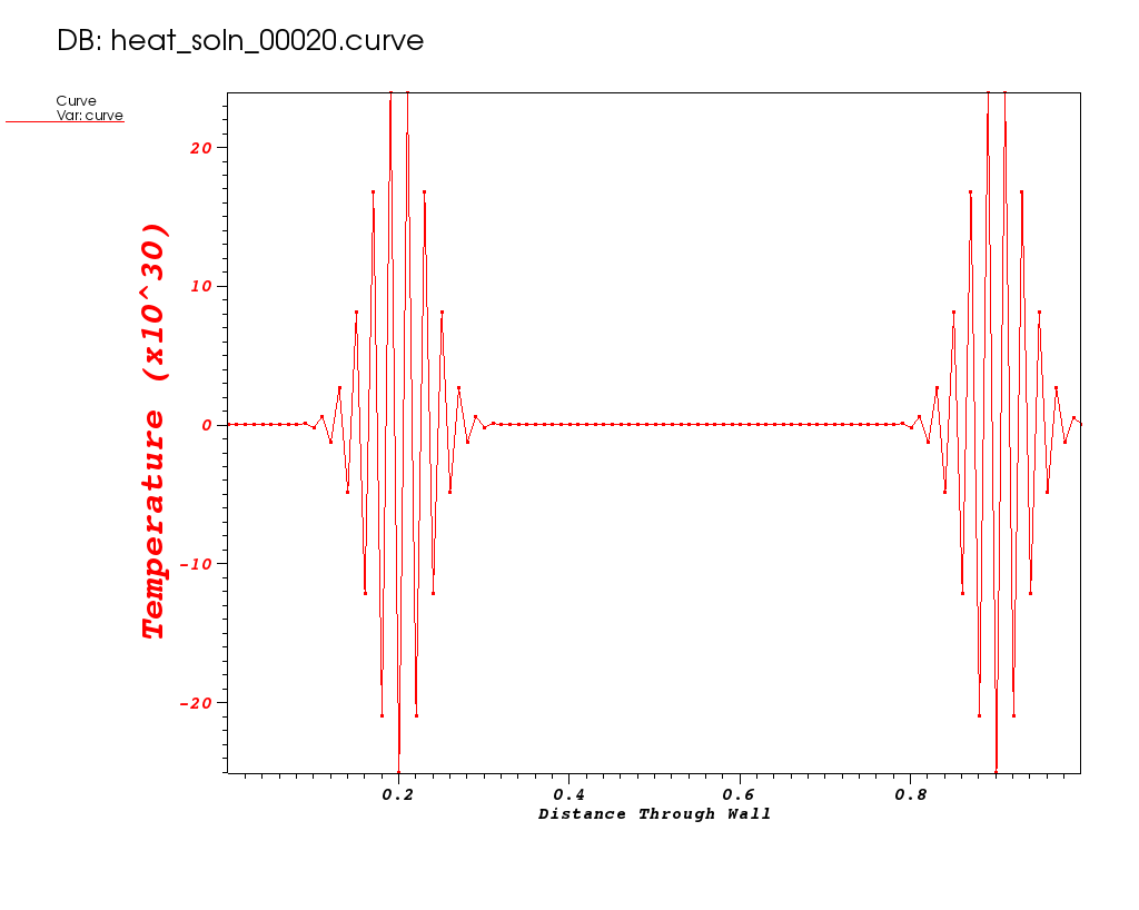Note the Y-axis range in these plots. It gets out of control!

What do you think happened?

This goes back to our original design choice in the method of discretization. That choice may not be appropriate for all of the science questions we want our application to be able to answer. In particular, the FTCS algorithm is known to have stability issues for certain combinations dt and dx.

What can we do to correct for the instability?

We can naively correct for this by shrinking the time-step.

Run 3

The FTCS algorithm is known to be stable only for values of r in equation 6 less than or equal to 1/2. Given a spatial resolution, dx=0.01, this means our timestep size now needs to be less than or equal to 0.00025. Lets run with a value of dt=0.0001.

$ make hr_spikes_smalldt
./heat dx=0.01 dt=0.0001 bc1=0 ic="spikes(10,20,10,90)" savi=500
    prec=double
    alpha=0.2
    dx=0.01
    dt=0.0001
    maxt=2
    bc0=0
    bc1=0
    ic=spikes(10,20,10,90)
    alg=ftcs
    savi=500
    save=0
    outi=100
    noout=0
Timestep 0000: last change l2=48
Timestep 0100: last change l2=0.000169428
Timestep 0200: last change l2=3.60231e-05
Timestep 0300: last change l2=1.35141e-05
Timestep 0400: last change l2=6.83466e-06
Timestep 0500: last change l2=4.08578e-06
.
.
.
Timestep 19800: last change l2=2.52461e-11
Timestep 19900: last change l2=2.42688e-11
Timestep 20000: last change l2=2.33386e-11
Integer ops        = 56755439
Floating point ops = 18165900
Memory used        = 1636 bytes

Plots from some early times in the run are shown below…

Time 0	Time 0.05	Time 0.1

Where do you estimate the local minimum occurs?

It appears to occur between 0.56 and 0.57.

Why did this run use more memory?

It is a more finely resolved mesh.

How many more flops were required?

18165900 on this more finely resolved mesh vs. 50310 on the coarse mesh. Thats 361x more flops!

The solution changes very slowly at late time. Do we need to use the same small timestep for all timesteps?

Not necessarily. But, how would you go about changing the method so that it could robustly adapt the timestep to changing conditions of the solution?

Can we achieve solution of similar quality with fewer flops?

Maybe. But, we probably need to consider a different discretization. Do we really want to have to support multiple different numerical methods in our application? Yet another advantage of using community adopted numerical packages is that such packages often provide a great deal of flexibility in choice of algorithm.

Crank-Nicolson Discretization

Using the Crank-Nicolson discretization, we arrive at the following discretization of equation 2…

$-ru_{i+1}^{k+1}+(1+2r)u_i^{k+1}-ru_{i-1}^{k+1} = ru_{i+1}^k+(1-2r)u_i^k+ru_{i-1}^k$

(7)

where $r= \alpha \frac{\Delta t}{2 \Delta x^2}$

In equation 7, the solution at spatial position i and time k+1 now depends not only on values of u at time k but also on other values of u at time k+1. This means each time we advance the solution in time we must solve a linear system; in other words we must solve for all of the values at time k+1 in one step. This is an example of an implicit method. In this case, the system of equations is tri-diagonal – since each update for u at i only uses u at i-1 , i and i+1 – so it is easier to implement than a general matrix solve but is still more complicated than an explicit update.

The code to implement this method is more involved because it involves doing a tri-diagonal solve.

/* Author: John Burkardt, 30May09 */
static void
init_and_factor_A_matrix(int n, double *a_lu,
    double alpha, double dt, double dx)
{
    int i;
    double r = alpha * dt / dx / dx / 2;

    a_lu[0+0*3] = 0.0;
    a_lu[1+0*3] = 1.0;
    a_lu[0+1*3] = 0.0;

    for ( i = 1; i < Nx - 1; i++ )
    {
        a_lu[2+(i-1)*3] =           - r;
        a_lu[1+ i   *3] = 1.0 + 2.0 * r;
        a_lu[0+(i+1)*3] =           - r;
    }

    a_lu[2+(Nx-2)*3] = 0.0;
    a_lu[1+(Nx-1)*3] = 1.0;
    a_lu[2+(Nx-1)*3] = 0.0;

    /* Factor the matrix.  */
    for ( i = 1; i <= n-1; i++ )
    {
        /* Store the multiplier in L.  */
        a_lu[2+(i-1)*3] = a_lu[2+(i-1)*3] / a_lu[1+(i-1)*3];

        /* Modify the diagonal entry in the next column.  */
        a_lu[1+i*3] = a_lu[1+i*3] - a_lu[2+(i-1)*3] * a_lu[0+i*3];
    }
}

static void r83_np_sl(int n,
    double const *a_lu, double const *last, double *curr)
{
    int i;

    for ( i = 0; i < n; i++ )
        curr[i] = last[i];

    /* Solve L * Y = B.  */
    for ( i = 1; i < n; i++ )
        curr[i] = curr[i] - a_lu[2+(i-1)*3] * curr[i-1];

    /* Solve U * X = Y.  */
    for ( i = n; 1 <= i; i-- )
    {
        curr[i-1] = curr[i-1] / a_lu[1+(i-1)*3];
        if ( 1 < i )
            curr[i-2] = curr[i-2] - a_lu[0+(i-1)*3] * curr[i-1];
    }

    /* Impose boundary conditions */
    curr[0  ] = bc0;
    curr[n-1] = bc1;
}

Here, we have code that sets up and LU factors the initial matrix. Then, the LU factored matrix is used on each solution timestep to solve for the new temperatures.

Run 4 (original dt=0.004)

$ make hr_spikes_crankn
./heat alpha= dx=0.01 bc1=0 ic="spikes(10,20,10,90)" alg=crankn savi=10
    prec=double
    alpha=0.2
    dx=0.01
    dt=0.004
    maxt=2
    bc0=0
    bc1=0
    ic=spikes(10,20,10,90)
    alg=crankn
    savi=10
    save=0
    outi=100
    noout=0
Timestep 0000: last change l2=148.274
Timestep 0100: last change l2=2.09991e-05
Timestep 0200: last change l2=4.24893e-06
Timestep 0300: last change l2=8.81289e-07
Timestep 0400: last change l2=1.82834e-07
Timestep 0500: last change l2=3.85324e-08
Integer ops        = 5809323
Floating point ops = 605800
Memory used        = 4067 bytes

Run 5 (larger dt=0.008)

$ make hr_spikes_crankn_largedt
./heat dx=0.01 dt=0.008 bc1=0 ic="spikes(10,20,10,90)" alg=crankn savi=5
    prec=double
    alpha=0.2
    dx=0.01
    dt=0.008
    maxt=2
    bc0=0
    bc1=0
    ic=spikes(10,20,10,90)
    alg=crankn
    savi=5
    save=0
    outi=100
    noout=0
Timestep 0000: last change l2=162.895
Timestep 0100: last change l2=1.69397e-05
Timestep 0200: last change l2=7.37902e-07
Timestep 0250: last change l2=1.58932e-07
Integer ops        = 4439568
Floating point ops = 303790
Memory used        = 4067 bytes

Why do these runs with Crank-Nicolson use more memory?

This is the memory required to store a banded matrix for the implicit solve. It is about 3x as much memory (for main diagonal and two sub-diagonals) over the FTCS method.

Is this algorithm better than FTCS?

It depends on what science you are trying to achieve. Here, the small timestep that the FTCS algorithm needs for stability makes it really expensive; we can get enough accuracy by instead using the Crank-Nicolson algorithm. On the other hand, the Crank-Nicolson approach requires greater memory usage and greater complexity in implementation.

How would you parallelize this algorithm…with threads, with MPI, with Cuda/GPU?

You need to break the tri-diagonal matrix into blocks on each processing element and exchange data between blocks. But, what if the matrix was not tri-diagonal?

Why Use Numerical Software Packages Instead of Hand Coding?

What if we want to plan the development of our application so we can easily enhance it later to support more complex situations such as…

More than just one spatial dimension
Coordinate systems other than just Cartesian
Heat sources
More complex materials
- A laminated material where each laminant has a different thermal diffusivity
- A material where thermal diffusivity is nonisotropic (e.g. different for different directions of heat flow).
- A material where thermal diffusivity may vary with either space, x, or event time, t.
- A material where thermal diffusivity may vary with temperature, u, introducing nonlinearities and the need for nonlinear solvers.
More complex domains
- Much larger objects involving billions of discretization points and requiring scalability in all phases of the solution.
- Domains that perehaps aren’t square and may have features with highly variable spatial resolutions requiring unstructured and/or adaptive meshing.
Parallelism and complex computational settings on high-performance architectures
- MPI+X
- GPU
- ARM
- Various parallel runtimes
Other aspects of modeling, simulation, and analytics
- Alternative models and domain-specific science details
- Multiphysics, multiscale, multidomain, multiresolution
- Work toward predictive simulation, optimization, and design
More agile and sustainable software, addressing
- Understandability of code, with encapsulation of complexities
- Robustness, efficiency, scalability, portability, reproducibility
- Ease of debugging
- Thorough testing
- Extensibility to exploit application-specific knowledge
- Interoperability with complementary software

Addressing these issues for large-scale simulations in science and engineering is one of the key values of numerical packages. Many of the details of these issues have been resolved and vetted within the scientific computing community within widely used software packages. Numerical packages can help to simplify the development of highly sophisticated scientific computing applications and provide a much more solid, flexible, and sustainable foundation than code that is completely written from scratch. Moreover, well-designed numerical software packages enable users to build custom solution strategies that leverage application-specific knowledge.

Out-Brief

We have demonstrated some of the tradeoffs in developing a custom-coded C application to model time-varying heat conduction in a wall. We developed two different numerical schemes, FTCS and Crank-Nicolson. The FTCS scheme is an explicit scheme whereas Crank-Nicolson is an implicit scheme. We demonstrated some of the attributes of these methods such as relative implementation complexity, memory usage, flop counts, and stability. Numerous other attributes of numerical algorithms will be introduced and discussed in later lessons.

We have explained some of the drawbacks of developing completely hand-coded solutions as well as some of the advantages of using community adopted numerical packages for application development.

The remainder of the lessons focus on the use of various software packages in the solution of ever more complex settings.

A simple examination of the C code, heat.c demonstrates that in spite of numerous simplifications we have made here, developing the code necessary to implement numerical algorithms and, in particular, to provide significant flexibility in the methods of solution and to understand and control their behavior is non-trivial. Code development can get quite complex very quickly.

HandsOnLessons

A github pages site hosting hands-on lessons in the use, design and development of scientific computing software packages