Sparse Direct Solver
At A Glance
Questions                  |Objectives                      |Key Points
---------------------------|--------------------------------|----------
Why need direct solver?    | Can obtain accurate solution   | Robust for difficult problems
What parameters affect     | Try different ordering options | Performance (time & memory)
performance?               |                                | can vary a lot
Note: To begin this lesson
cd handson/mfem/examples/atpesc/superlu
The problem being solved
The convdiff.c application is modeling the steady state convection-diffusion equation in 2D with a constant velocity. This equation is used to model the concentration of something like a die in a moving fluid as it diffuses and flows through he fluid. The equation is as follows:
| (1) |
Where u is the concentration that we are tracking,
is the diffusion rate,
v is the velocity of the flow and R is a concentration source.
In the application we use here, the velocity vector direction is fixed in the +x
direction. However, the magnitude is set by the user (default of 100),
is fixed at 1.0, and the
source is 0.0 everywhere except for a small disc centered at the middle of the
domain where it is 1.0.
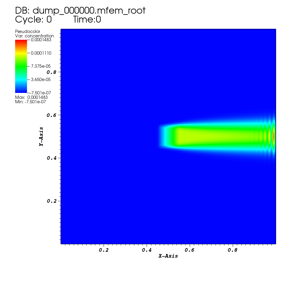
| Initial Condition |
|---|
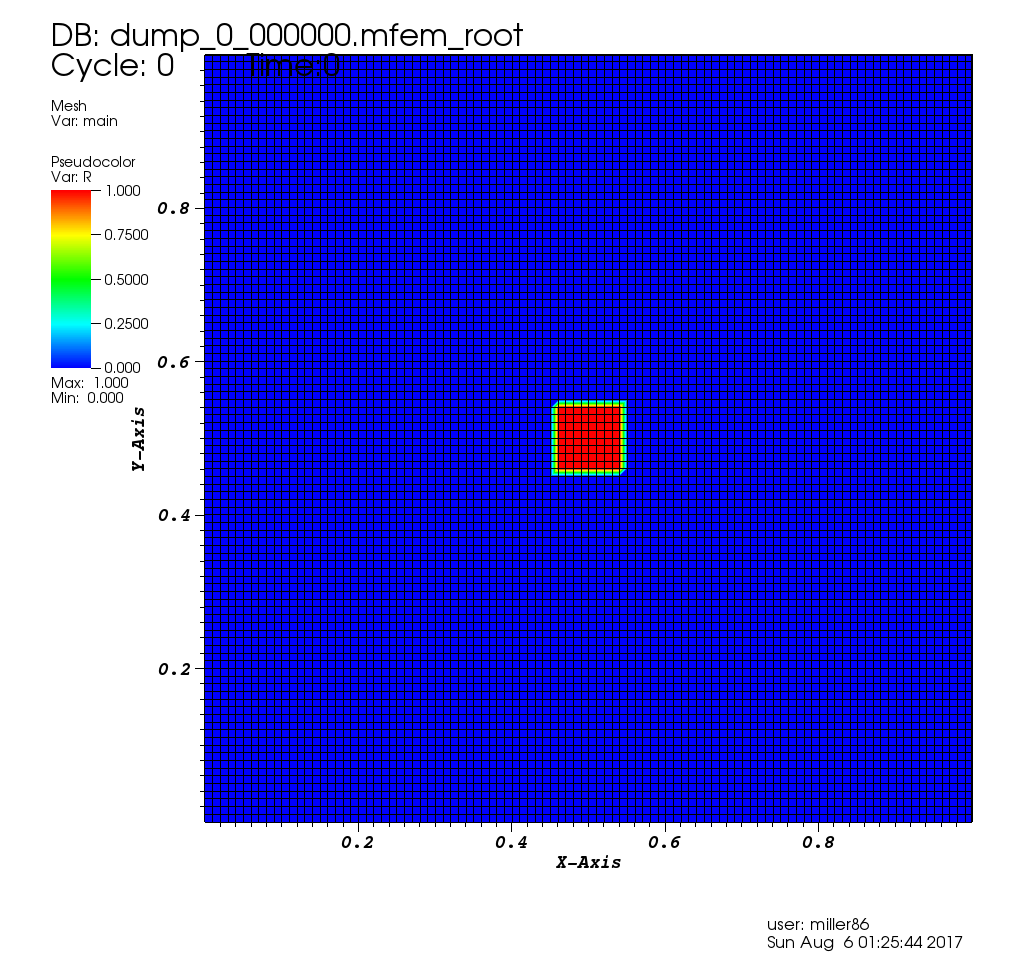 |
Solving this PDE is well known to cause convergence problems for iterative solvers, for larger v. We use MFEM as a vehicle to demonstrate the use of a distributed, direct solver, SuperLU_DIST, to solve very ill-conditioned linear systems.
The Example Source Code
Running the Example
Run 1: default setting with GMRES solver, preconditioned by hypre, velocity = 100
$ ./convdiff

Options used:
   --refine 0
   --order 1
   --velocity 100
   --no-visit
   --no-superlu
   --slu-colperm 0
Number of unknowns: 10201
=============================================
Setup phase times:
=============================================
GMRES Setup:
  wall clock time = 0.010000 seconds
  wall MFLOPS     = 0.000000
  cpu clock time  = 0.010000 seconds
  cpu MFLOPS      = 0.000000

L2 norm of b: 9.500000e-04
Initial L2 norm of residual: 9.500000e-04
=============================================

Iters     resid.norm     conv.rate  rel.res.norm
-----    ------------    ---------- ------------
    1    4.065439e-04    0.427941   4.279409e-01
    2    1.318995e-04    0.324441   1.388415e-01
    3    4.823031e-05    0.365660   5.076874e-02
    ...
   23    2.436775e-16    0.249025   2.565027e-13

Final L2 norm of residual: 2.436857e-16

=============================================
Solve phase times:
=============================================
GMRES Solve:
  wall clock time = 0.030000 seconds
  wall MFLOPS     = 0.000000
  cpu clock time  = 0.020000 seconds
  cpu MFLOPS      = 0.000000

GMRES Iterations = 23
Final GMRES Relative Residual Norm = 2.56511e-13
Time required for solver:  0.0362886 (s)
| Steady State |
|---|
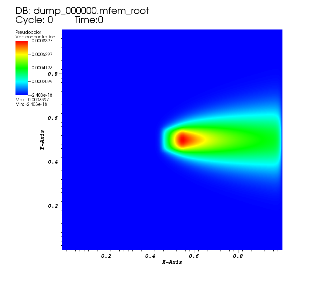 |
Run 2: increase velocity to 1000, GMRES does not converge anymore
$ ./convdiff --velocity 1000

Options used:
   --refine 0
   --order 1
   --velocity 1000
   --no-visit
   --no-superlu
   --slu-colperm 0
Number of unknowns: 10201
=============================================
Setup phase times:
=============================================
GMRES Setup:
  wall clock time = 0.020000 seconds
  wall MFLOPS     = 0.000000
  cpu clock time  = 0.010000 seconds
  cpu MFLOPS      = 0.000000

L2 norm of b: 9.500000e-04
Initial L2 norm of residual: 9.500000e-04
=============================================

Iters     resid.norm     conv.rate  rel.res.norm
-----    ------------    ---------- ------------
    1    9.500000e-04    1.000000   1.000000e+00
    2    9.500000e-04    1.000000   1.000000e+00
    3    9.500000e-04    1.000000   1.000000e+00
    ...
  200    9.500000e-04    1.000000   1.000000e+00
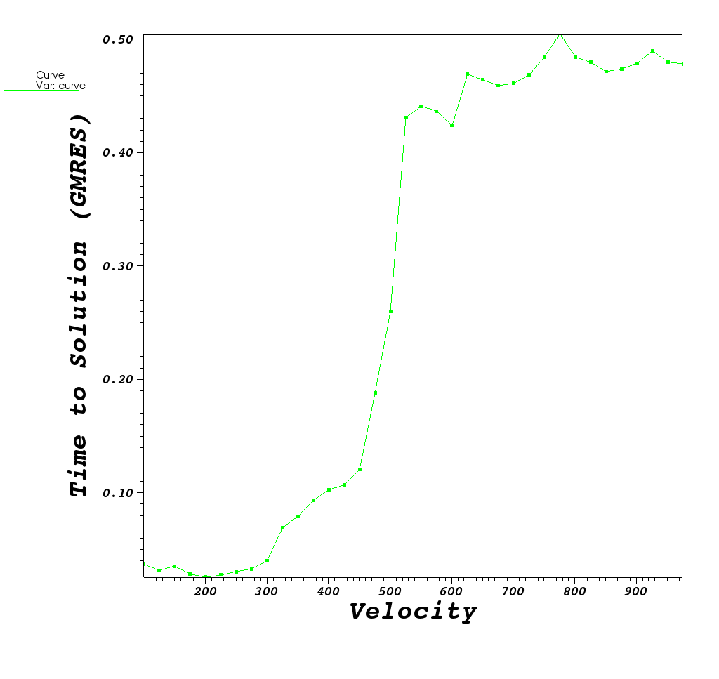
Below, we plot behavior of the GMRES method for velocity values in the range [100,1000] at incriments, dv, of 25 and also show an animation of the solution GMRES gives as velocity increases
| Solutions @dv=25 in [100,1000] | Contours of Solution @ vel=1000 |
|---|---|
 |
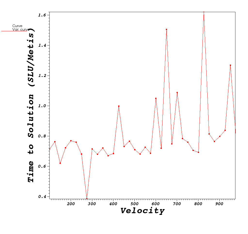
| Time to Solution | L2 norm of final residual |
|---|---|
 |
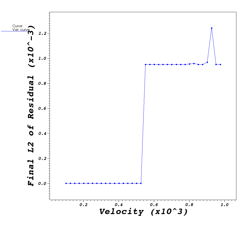 |
What do you think is happening?
| GMRES method works ok for low velocity values. As velocity increases, GMRES method eventually crosses a threshold where it can no longer provide a useful result. |
Why does time to solution show smoother transition than L2 norm?
| As instability is approached, more GMRES iterations are required to reach desired norm. So GMRES is still able to manage the solve and achieve a near-zero L2 norm. It just takes more and more iterations. Once GMRES is unable to solve the L2 norm explodes. |
Run 3: Now use SuperLU_DIST, with default options
$ ./convdiff -slu --velocity 1000

Options used:
   --refine 0
   --order 1
   --velocity 1000
   --no-visit
   --superlu
   --slu-colperm 0
Number of unknowns: 10201

** Memory Usage **********************************
** NUMfact space (MB): (sum-of-all-processes)
    L\U :           41.12 |  Total :    50.72
** Total highmark (MB):
    Sum-of-all :    62.27 | Avg :    62.27  | Max :    62.27
**************************************************
Time required for solver:  38.2684 (s)
Final L2 norm of residual: 1.55553e-18
| Stead State For vel=1000 |
|---|
 |
Run 4: Now use SuperLU_DIST, with MMD(A’+A) ordering.
$ ./convdiff -slu --velocity 1000 --slu-colperm 2

Options used:
   --refine 0
   --order 1
   --velocity 1000
   --no-visit
   --superlu
   --slu-colperm 2
Number of unknowns: 10201
       Nonzeros in L       594238
       Nonzeros in U       580425
       nonzeros in L+U     1164462
       nonzeros in LSUB    203857

** Memory Usage **********************************
** NUMfact space (MB): (sum-of-all-processes)
    L\U :           10.07 |  Total :    16.19
** Total highmark (MB):
    Sum-of-all :    16.19 | Avg :    16.19  | Max :    16.19
**************************************************
Time required for solver:  0.780516 (s)
Final L2 norm of residual: 1.52262e-18
NOTE: the number of nonzeros in L+U is much smaller than natural ordering. This affects the memory usage and runtime.
Run 5: Now use SuperLU_DIST, with Metis(A’+A) ordering.
$ ./convdiff -slu --velocity 1000 --slu-colperm 4

Options used:
   --refine 0
   --order 1
   --velocity 1000
   --no-visit
   --superlu
   --slu-colperm 4
Number of unknowns: 10201
       Nonzeros in L       522306
       Nonzeros in U       527748
       nonzeros in L+U     1039853
       nonzeros in LSUB    218211

** Memory Usage **********************************
** NUMfact space (MB): (sum-of-all-processes)
    L\U :            9.24 |  Total :    15.64
** Total highmark (MB):
    Sum-of-all :    15.64 | Avg :    15.64  | Max :    15.64
**************************************************
Time required for solver:  0.786936 (s)
Final L2 norm of residual: 1.55331e-18
| Solutions @dv=25 in [100,1000] | Steady State Solution @ vel=1000 |
|---|---|
|
| Time to Solution |
|---|
 |
Run 6: Now use SuperLU_DIST, with Metis(A’+A) ordering, using 16 MPI tasks, on a larger problem.
By adding --refine 2, each element in the mesh is subdivided twice yielding a 16x larger problem.
Here, we’ll run on 16 tasks and just grep the output form some key values of interest.
$ ${MPIEXEC_OMPI} -n 16 ./convdiff --refine 2 --velocity 1000 -slu --slu-colperm 4 >& junk.out
$ grep 'Time required for solver:' junk.out
Time required for solver:  10.3593 (s)
Time required for solver:  16.3567 (s)
Time required for solver:  11.6391 (s)
Time required for solver:  10.669 (s)
Time required for solver:  10.0605 (s)
Time required for solver:  10.1216 (s)
Time required for solver:  20.0721 (s)
Time required for solver:  10.6205 (s)
Time required for solver:  13.8445 (s)
Time required for solver:  11.8943 (s)
Time required for solver:  16.1552 (s)
Time required for solver:  13.0849 (s)
Time required for solver:  14.0008 (s)
Time required for solver:  13.238 (s)
Time required for solver:  12.387 (s)
Time required for solver:  9.81836 (s)
$ grep 'Final L2 norm of residual:' junk.out
Final L2 norm of residual: 3.06951e-18
Final L2 norm of residual: 3.06951e-18
Final L2 norm of residual: 3.06951e-18
Final L2 norm of residual: 3.06951e-18
Final L2 norm of residual: 3.06951e-18
Final L2 norm of residual: 3.06951e-18
Final L2 norm of residual: 3.06951e-18
Final L2 norm of residual: 3.06951e-18
Final L2 norm of residual: 3.06951e-18
Final L2 norm of residual: 3.06951e-18
Final L2 norm of residual: 3.06951e-18
Final L2 norm of residual: 3.06951e-18
Final L2 norm of residual: 3.06951e-18
Final L2 norm of residual: 3.06951e-18
Final L2 norm of residual: 3.06951e-18
Final L2 norm of residual: 3.06951e-18
Can you explain the processor times relative to the previous, single processor run?
| We've increased the mesh size by 16x here. But, we've also added 16x processors. Yet, the time for those processors to run ranged between 10 and 20 seconds with an average of 12.7 seconds. The smaller, single processor run took 0.786936 and taking the ratio of these numbers, we get ~16. However, recall that the matrix size goes up as the SQUARE of the mesh size and this accounts for this additional factor of 16. |
Out-Brief
In this lesson, we have used MFEM as a vehicle to demonstrate the value of direct solvers from the SuperLU_DIST numerical package.
Further Reading
To learn more about sparse direct solver, see Gene Golub SIAM Summer School course materials: Lecture Notes, Book Chapter, and Video