Time Integration
Time Integration with SUNDIALS
At a Glance
| Questions | Objectives | Key Points |
| How do explicit, implicit or IMEX methods impact step size? | Compare methods at step sizes near the stability limit. | Choose time integration method to match the problem. |
| What is the impact of an adaptive technique? | Compare fixed and adaptive techniques. | Adaptive techniques can be robust reliable and reduce computational cost. |
| How does integration order impact cost? | Observe impact of order on time to solution and number of steps. | Changing integration order is simple allowing optimization for a given problem. |
| What is the role and benefit of preconditioning? | Compare integration methods with and without preconditioning. | Preconditioning is critical for scalability. |
Setup Instructions
-
Make sure that you have followed the setup instructions
- Change to the directory containing the precompiled executables, input files,
and post processing scripts for this lesson:
cd track-5-numerical/time_integration_sundials - For postprocessing output files load and activate conda:
module load conda
conda activate base
The entire set of hands-on lesson codes is also available on
GitHub, under the
SUNDIALS+AMReX directory.
The Problem Being Solved
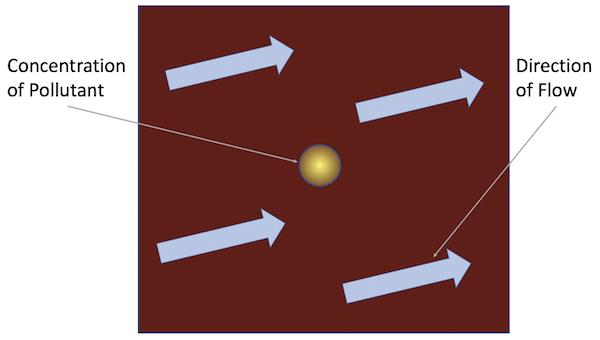
In this problem, we model the transport of a pollutant that has been released into a flow in a two dimensional domain. We want to determine both where the pollutant goes, and when it has diffused sufficiently to be of no further harm.
This is an example of a scalar-valued advection-diffusion problem for chemical transport. The governing equation is: \[\frac{\partial u}{\partial t} + \vec{a} \cdot \nabla u - \nabla \cdot ( D \nabla u ) = 0\]
where \(u = u(t,x,y)\) is the chemical concentration, \(\vec{a}\) is the advection vector, \(D\) is a diagonal matrix containing anisotropic diffusion coefficients, and \(u(0,x,y)=u_0(x,y)\) is a given initial condition. The spatial domain is \((x,y) \in [-1,1]^2,\) and the time domain is \(t \in (0,10^4].\)
The Application Models
The example application uses a finite volume spatial discretization with AMReX. For the time integration (i.e., semi-discretization in time) of this PDE, we use the ARKODE ODE integrator from SUNDIALS, to demonstrate the use of SUNDIALS with CUDA parallelism for more robust and flexible control over temporal integration.
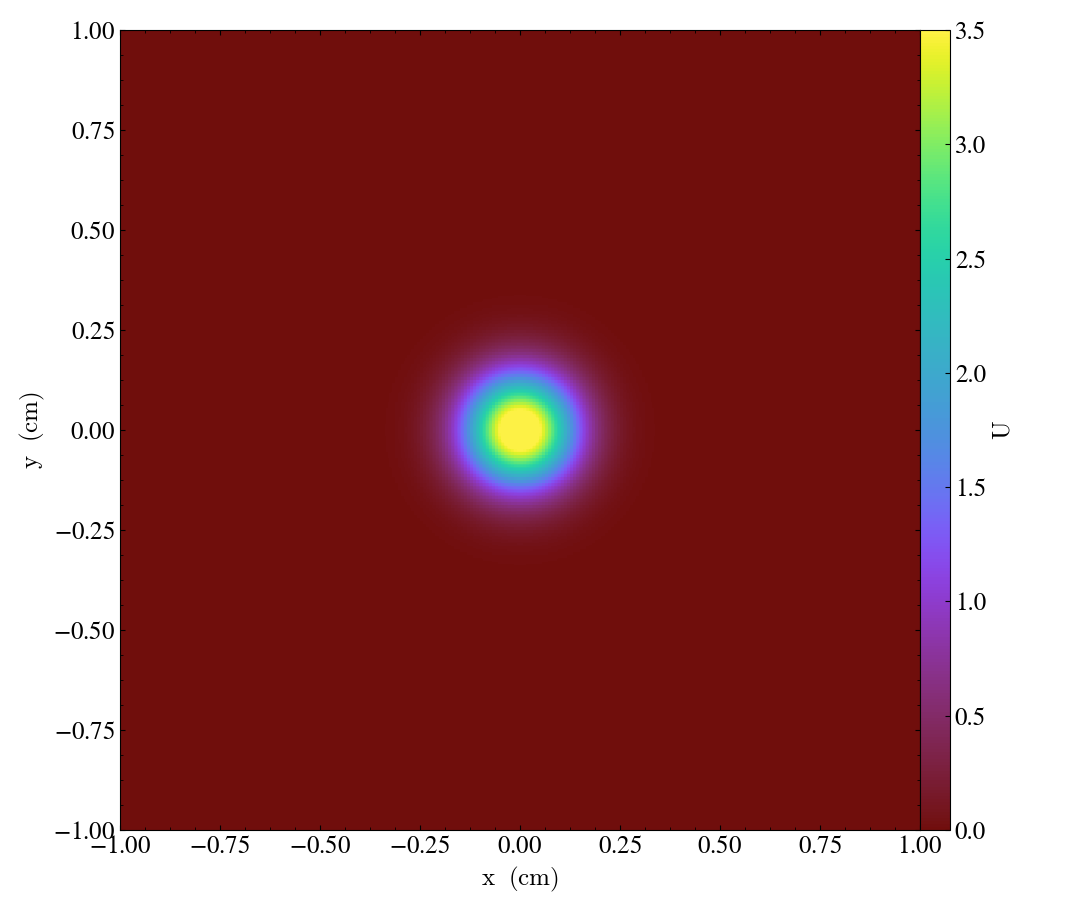
Each application solves the problem on a periodic, cell-centered, uniform mesh with an initial Gaussian bump: \[u_0(x,y) = \frac{10}{\sqrt{2\pi}} e^{-50(x^2+y^2)}.\]
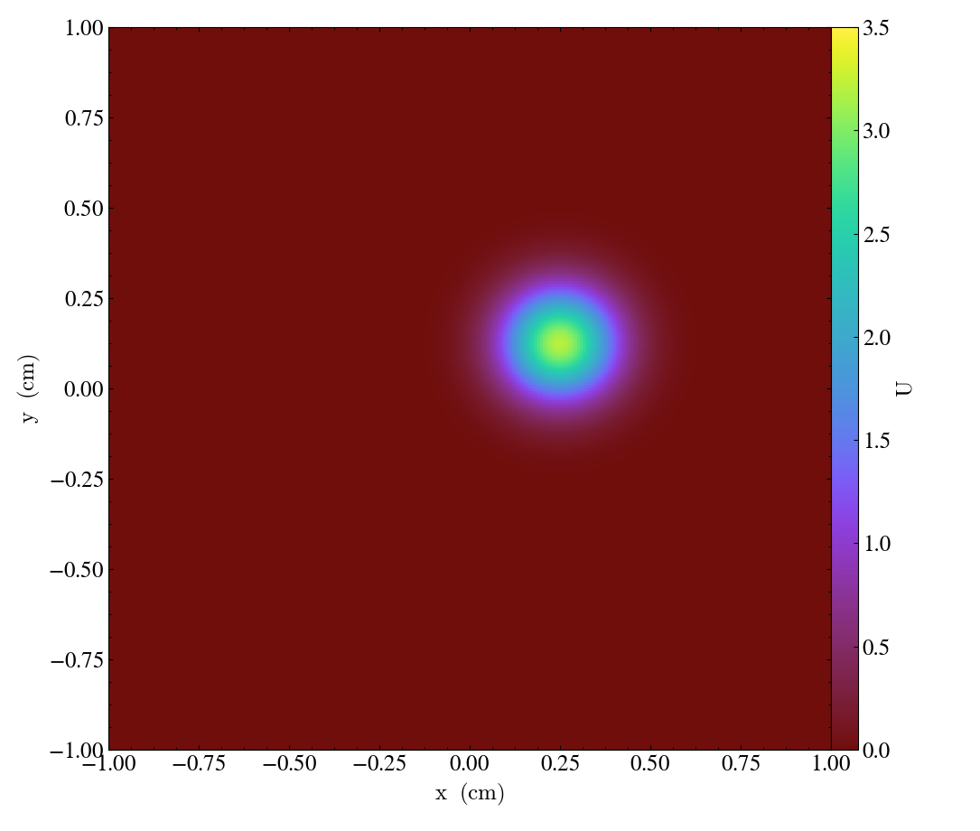
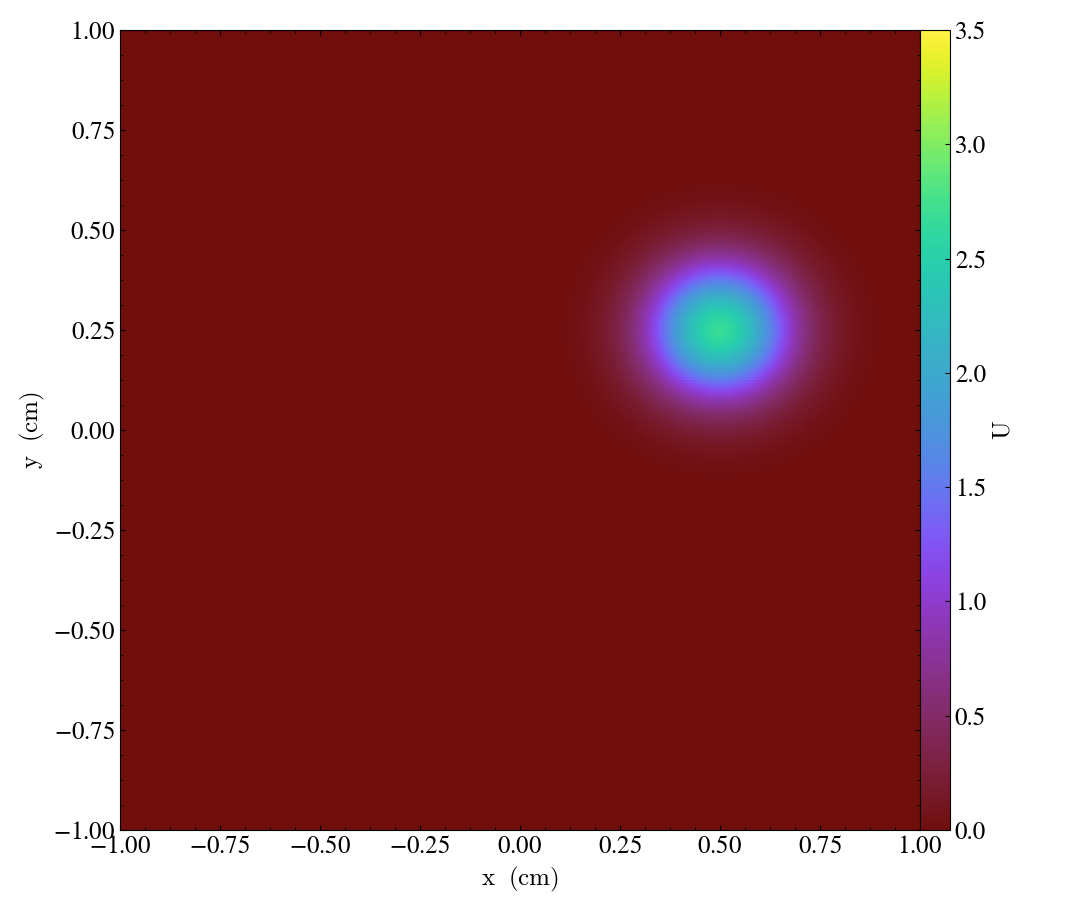
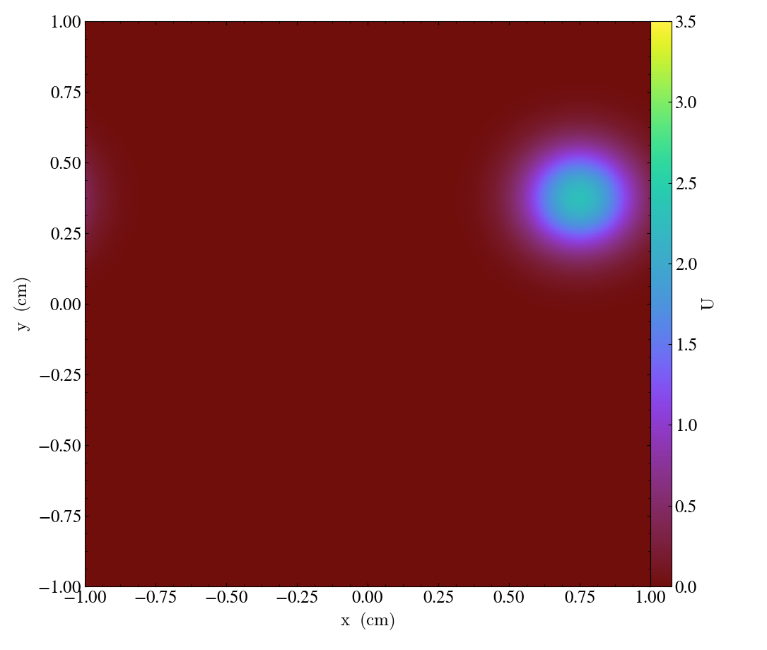
Snapshots of the solution for the advection [flow] vector \(\vec{a}=\left[ 0.0005,\, 0.00025\right],\) and diffusion coefficient matrix \(D = \operatorname{diag}\left(\, \left[10^{-6},\, 10^{-6}\right]\,\right)\) at the times \(t = \left\{0, 1000, 2000, 3000\right\}\) are shown in Figures 1-4 below:
| Figure 1 | Figure 2 | Figure 3 | Figure 4 |
|---|---|---|---|
| 
| 
| 
|
We will investigate this problem in three phases:
-
Explicit time integration (HandsOn1.cpp,
HandsOn1.CUDA.exe) -
Implicit / implicit-explicit (IMEX) time integration (HandsOn2.cpp,
HandsOn2.CUDA.exe) -
Preconditioning (HandsOn3.cpp,
HandsOn3.CUDA.exe– optional)
Getting Help
You can discover the full set of command-line options for each setup with
the help=1 argument, e.g.,
mpiexec -n 1 ./HandsOn1.CUDA.exe help=1
which should produce output like the following:
Initializing AMReX (24.08)...
MPI initialized with 1 MPI processes
MPI initialized with thread support level 0
Initializing CUDA...
CUDA initialized with 1 device.
Initializing SUNDIALS with 1 threads...
SUNDIALS initialized.
AMReX (24.08) initialized

Usage: HandsOn1.exe [fname] [options]
Options:
  help=1
    Print this help message and exit.
  plot_int=<int>
    enable (1) or disable (0) plots [default=0].
  arkode_order=<int>
    ARKStep method order [default=4].
  fixed_dt=<float>
    use a fixed time step size (if value > 0.0) [default=-1.0].
  rtol=<float>
    relative tolerance for time step adaptivity [default=1e-4].
  atol=<float>
    absolute tolerance for time step adaptivity [default=1e-9].
  tfinal=<float>
    final integration time [default=1e4].
  dtout=<float>
    time between outputs [default=tfinal].
  max_steps=<int>
    maximum number of internal steps between outputs [default=10000].
  write_diag=<int>
    output ARKStep time step adaptivity diagnostics to a file [default=1].
  n_cell=<int>
    number of cells on each side of the square domain [default=128].
  max_grid_size=<int>
    max size of boxes in box array [default=64].
  advCoeffx=<float>
    advection speed in the x-direction [default=5e-4].
  advCoeffy=<float>
    advection speed in the y-direction [default=2.5e-4].
  diffCoeffx=<float>
    diffusion coefficient in the x-direction [default=1e-6].
  diffCoeffy=<float>
    diffusion coefficient in the y-direction [default=1e-6].

If a file name 'fname' is provided, it will be parsed for each of the above
options.  If an option is specified in both the input file and on the
command line, then the command line option takes precedence.
Hands-on Lesson 1 – Explicit Time Integration
This lesson uses HandsOn1.CUDA.exe and explores the following topics:
a. Problem specification – vector wrapper and right-hand side functions
b. Fixed time-stepping (exploration of linear stability)
c. Adaptive time-stepping
d. Time integrator order of accuracy
Problem Specification
There are essentially only three steps required to use SUNDIALS with an existing simulation code:
-
Create an
N_Vectorwrapper for your application data structures, so that SUNDIALS can perform standard vector operations directly on your data.AMReX provides an
N_Vectorimplementation wrapping its nativeMultiFabdata structure (see the files AMReX_NVector_MultiFab.H and AMReX_NVector_MultiFab.cpp in the AMReX repository).This vector implements the vector operations need by SUNDIALS (linear combination \(\vec{z} \gets a\vec{x} + b\vec{y}\), inner-product \(\left<\vec{x},\vec{y}\right>\), etc.) and leverages the native
MultiFaboperations andamrex::ParallelForto perform the computations on the CPU or GPU. -
Create a function that computes the problem-defining ODE right-hand side function. In this example, we implement the advection-diffusion right-hand side function, \[f(t,u) = -\vec{a} \cdot \nabla u + \nabla \cdot ( D \nabla u )\]
in the file HandsOn_main.cpp as
int ComputeRhsAdvDiff(Real t, N_Vector nv_sol, N_Vector nv_rhs, void* data)This function utilizes the AMReX
amrex::ParallelForto execute the computations the CPU or offload the work to the GPU. -
Use SUNDIALS to integrate your ODE/DAE:
-
Instantiate and fill an
N_Vectorfor the initial condition, \(u_0(x,y)\). In our example this is done here inHandsOn_main.cpp. -
Create the time integrator, providing both the initial condition vector \(u_0(x,y)\) and the problem-defining function \(f(t,u)\). In our example, this is done here in
HandsOn1.cpp. -
Call the SUNDIALS integrator to evolve the problem over a series of out time intervals. Our example does this in a loop here in
HandsOn1.cpp.
-
Linear Stability
Run the first hands-on code using its default parameters (note that this uses a mesh size of \(128^2\) and fixed time step size of 5.0),
mpiexec -n 4 ./HandsOn1.CUDA.exe inputs-1
and compare the final result against a stored reference solution (again on a \(128^2\) grid),
./amrex_fcompare plt00001/ reference_solution/
Notice that the computed solution error is rather small (the solution has magnitude \(\mathcal{O}(1)\), so we hope for errors well below 0.1).
Now re-run this hands-on code using a larger time step size of 25.0,
mpiexec -n 4 ./HandsOn1.CUDA.exe inputs-1 fixed_dt=25.0
the code now runs much faster. However, if we check the accuracy of the computed solution,
./amrex_fcompare plt00001/ reference_solution/
we see it has an incredibly large error (mine was \(\mathcal{O}(10^{98})\)).
At this mesh size, the explicit algorithm is unstable for a time step size of 25, but is stable for a time step size of 5.
Run the code a few more times, trying to identify the largest stable time step size.
Temporal Adaptivity
With this executable, we may switch to adaptive time-stepping (with the default
tolerances, \(rtol=10^{-4}\) and \(atol=10^{-9}\)) by specifying fixed_dt=0,
mpiexec -n 4 ./HandsOn1.CUDA.exe inputs-1 fixed_dt=0
./amrex_fcompare plt00001/ reference_solution/
note how rapidly the executable finishes, providing a solution that is both stable and accurate to within the specified tolerances!
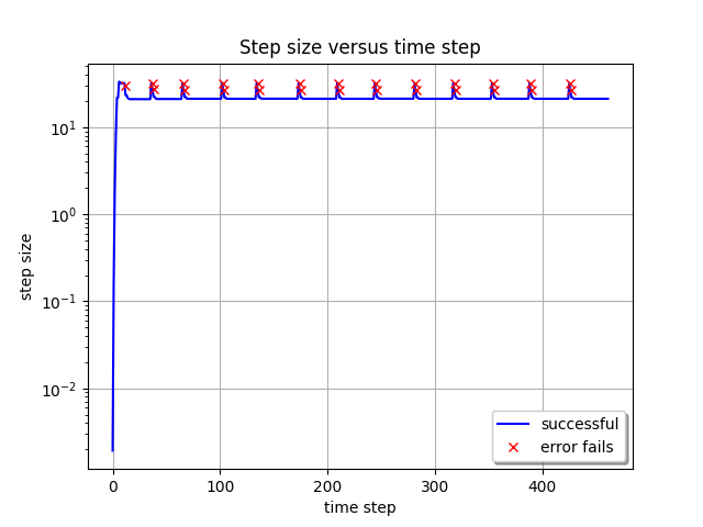
The time step sizes taken by the integrator in this run are seen below:
notice how rapidly the adaptive time-stepper finds the CFL stability limit. Also notice that the adaptivity algorithm periodically attempts to increase the time step size to investigate whether this stability limit has changed; however, the raw percentage of these failed steps remains rather small.
Note: You can generate the above plot by runing the provided Python script process_ARKStep_diags.py:
./process_ARKStep_diags.py HandsOn1_diagnostics.txt
We included it here because it can be difficult to display graphics from the GPU compute nodes on Polaris.
Run the code a few more times with various values of rtol (e.g.,
mpiexec -n 4 ./HandsOn1.CUDA.exe inputs-1 fixed_dt=0 rtol=1e-6) – how well does the adaptivity
algorithm produce solutions within the desired tolerances? How do the number of
time steps change as different tolerances are requested?
Integrator Order and Efficiency
ARKODE defaults to a fourth-order accurate Runge–Kutta method, but many others
are included (explicit methods have available orders 2 through 8). Alternate
orders of accuracy may be run with the arkode_order option, e.g.,
mpiexec -n 4 ./HandsOn1.CUDA.exe inputs-1 fixed_dt=0 arkode_order=8
./amrex_fcompare plt00001/ reference_solution/
note the dramatic decrease in overall time steps (462 vs 260), but the accompanying increase in total RHS evaluations (2413 vs 3759). Although higher-order methods may indeed utilize larger step sizes (both for accuracy and frequently stability), those come at the cost of increased work per step.
Run the code a few more times with various values of arkode_order for a fixed
value of rtol – what is the most “efficient” overall method for this problem
at this tolerance?
Hands-on lesson 2 – Implicit / IMEX Time Integration
This lesson uses HandsOn2.CUDA.exe and explores the following topics:
-
Specification of algebraic solver algorithms (nonlinear and linear)
-
Fixed time-stepping (exploration of linear stability)
-
Adaptive time-stepping
-
Implicit-explicit partitioning
Specification of Algebraic Solvers
Once your code is set up to run an explicit method, it is not difficult to
switch to an implicit or IMEX integrator. All of the relevant changes for this
in are in the file HandsOn2.cpp, and are indicated by the comment
***** UPDATED FROM HandsOn1 *****. The main steps are:
-
Move specification of the ODE right-hand side function to the implicit argument when creating the integrator, or supply separate routines that should be used for the IMEX splitting of the ODE right-hand side.
This is done here in
HandsOn2.cpp, where we either supply one functionComputeRhsAdvDiff()for fully implicit integration, or we supply two functions,ComputeRhsAdv()andComputeRhsDiff(), for an IMEX splitting of the ODE right-hand side. -
The default Newton nonlinear solver requires the user specify a linear solver for solving the inner linear system of equations for the Newton update.
In this example, we create and attach an un-preconditioned GMRES iterative linear solver here in
HandsOn2.cpp.
Linear Stability Revisited
Run the second hands-on code using its default parameters (this also uses a mesh size of \(128^2\) and fixed time step size of 5.0),
mpiexec -n 4 ./HandsOn2.CUDA.exe inputs-2
./amrex_fcompare plt00001/ reference_solution/
note that this takes significantly longer than HandsOn1.CUDA.exe with the
same time step size.
Re-run this problem using the larger time step size of 100.0,
mpiexec -n 4 ./HandsOn2.CUDA.exe inputs-2 fixed_dt=100.0
./amrex_fcompare plt00001/ reference_solution/
again this version runs much more quickly, but now the results are usable!
This algorithm is fully-implicit (and in fact, it is A-stable), so linear instability was not a problem.
Run the code a few more times with larger time step sizes, checking the overall solution error each time – can you find an unstable step size? Are there step sizes where the code may be stable, but are so large that the nonlinear and/or linear solver fails to converge?
Temporal Adaptivity Revisited
As with the previous hands-on exercise, we can switch to adaptive time-stepping
(with tolerances \(rtol=10^{-4}\) and \(atol=10^{-9}\)) by specifying
fixed_dt=0,
mpiexec -n 4 ./HandsOn2.CUDA.exe inputs-2 fixed_dt=0
Compute the solution error as before,
./amrex_fcompare plt00001/ reference_solution/
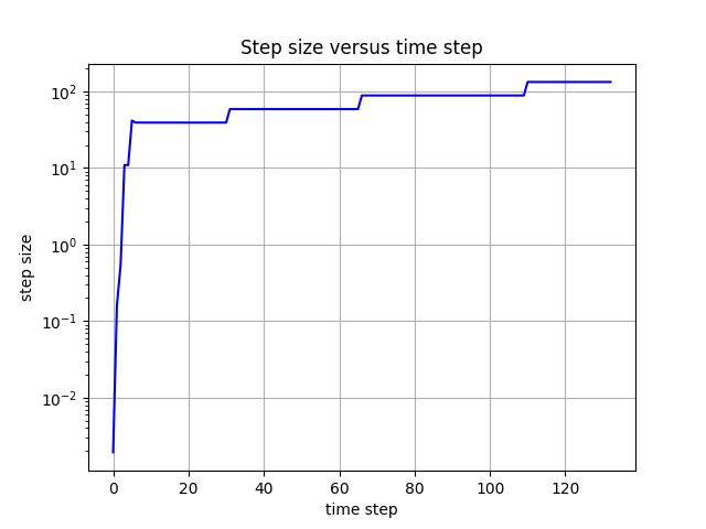
The corresponding time adaptivity history plot is below:
How does the average step size for this tolerance compare against the average
step size of HandsOn1.CUDA.exe for the same tolerances?
The solution becomes smoother and decays toward zero as time goes on. Since the solution changes more gradually as time proceeds, the integrator can ramp up the step size.
Run the code a few more times with various values of rtol – how well does the
adaptivity algorithm produce solutions within the desired tolerances? How do the
number of time steps change as different tolerances are requested? Is this
algorithm more useful than the fully explicit approach when loose tolerances
(e.g., rtol=1e-1) are requested?
IMEX Partitioning
By default, HandsOn2.CUDA.exe uses a fully implicit formulation of the problem.
However, this can instead be run with the advection terms
\(\vec{a} \cdot \nabla u\) treated explicitly by specifying rhs_adv=1, i.e.
mpiexec -n 4 ./HandsOn2.CUDA.exe inputs-2 rhs_adv=1
./amrex_fcompare plt00001/ reference_solution/
For comparison, re-run an identical test but with fully-implicit treatment,
mpiexec -n 4 ./HandsOn2.CUDA.exe inputs-2
./amrex_fcompare plt00001/ reference_solution/
Do you notice any efficiency or accuracy differences between fully implicit and IMEX formulations with these fixed time-step tests?
Since the explicit portion need only be computed once per
stage, but the implicit portion must be repeatedly called at each
stage during the nonlinear solver algorithm, we should expect
IMEX methods to always evalute Fi more often than Fe.
Now that we again have an explicit portion of the problem, we should expect the
time step size to be CFL-limited. Run the IMEX version a few times with various
fixed time step sizes (the fixed_dt argument), checking the overall solution
error each time – can you find a maximum stable step size?
Since diffusion is now treated implicitly, the CFL-limited step size is now determined only by the advection terms. As these are qualitatively different than the diffusion terms, we should expect different stability limitations.
We can again run the code using adaptive time stepping,
mpiexec -n 4 ./HandsOn2.CUDA.exe inputs-2 rhs_adv=1 fixed_dt=0
./amrex_fcompare plt00001/ reference_solution/
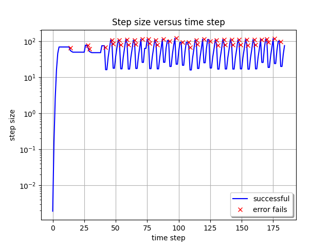
The corresponding stepsize history plot with this configuration is below, and shows similar behavior as we saw with the explicit method above.
Out-brief
We have used AMReX and SUNDIALS as a demonstration vehicle for illustrating the
value of robust time integration methods in numerical algorithms. In particular,
we have used ARKODE’s ARKStep time integration module from SUNDIALS to
explore a range of questions related to time integration and nonlinear solvers:
-
the benefits of adaptive (vs fixed) time stepping for both performance and robustness of a simulation code,
-
the effects of the order of the time integration method on method efficiency,
-
the choice of IMEX partitioning in time discretization.
We note that our use of adaptivity here was confined to the time discretization only. Other ATPESC lecturers demonstrate the advantages of spatial adaptation as well (e.g., AMR).
We further note that we have barely scratched the surface of algebraic linear solver algorithms; other of today’s ATPESC lecturers focus specifically on scalable and robust versions of these algorithms.
Finally, we note that the application demonstrated here can be run on much larger spatial meshes and parallel architectures than we have used in this demo.
Evening Hands-on Session – Preconditioning
This lesson uses HandsOn3.CUDA.exe to explore the following topics:
-
Preconditioner specification
-
Performance for IMEX time integrators
-
Performance for fully implicit time integrators
Preconditioner Specification
The file HandsOn3.cpp is nearly identical to the last example (with relevant
changes indicated by the comment ***** UPDATED FROM HandsOn2 *****), however,
its default parameters differ slightly:
-
it defaults to adaptive time-stepping (with the same default tolerances)
-
it defaults to IMEX mode, with advection treated explicitly
-
it defaults to using a preconditioner (discussed below).
Perhaps the most challenging (and most critical) component for a scalable implicit or IMEX time integrator is the creation of an effective, efficient, and scalable preconditioner to accelerate the iterative linear solvers (more on this by other ATPESC speakers). Use of a preconditioner with SUNDIALS requires two steps:
-
Create preconditioner “setup” and “solve” routines that prepare any data structures necessary to perform preconditioning (called infrequently) and apply the preconditioner (called frequently), respectively.
Here, we omit the setup function and provide a preconditioner_solve function, that employs a scalable geometric multigrid solver for only the diffusion portion of the problem, \(\nabla \cdot ( D \nabla u )\). This should be a perfect preconditioner when running in IMEX mode, but will only be approximate when running a fully implicit formulation of the problem.
-
Supply the preconditioning routines to the integrator.
In our example, when creating the GMRES linear solver, we signal to use left preconditioning here. We then attach the
precondition_solveroutine to the integrator here.
Performance with IMEX Integration
Run HandsOn3.CUDA.exe using the default parameters,
mpiexec -n 4 ./HandsOn3.CUDA.exe inputs-3
and again with preconditioning disabled,
mpiexec -n 4 ./HandsOn3.CUDA.exe inputs-3 use_preconditioner=0
Note that the preconditioned version takes longer to run on this coarse problem, but shows significant improvements in the overall number of linear solver iterations. However, as the mesh is refined the preconditioned solver performance will remain relatively “steady”, while the un-preconditioned solver will deteriorate rapidly.
Performance with Fully Implicit Integration
Re-run HandsOn3.CUDA.exe using a fully-implicit problem formulation,
mpiexec -n 4 ./HandsOn3.CUDA.exe inputs-3 rhs_adv=1
Recall that this preconditioner only “preconditions” the diffusion portion of the problem, so when run in a fully-implicit manner the implicit advection terms are left un-preconditioned. Is this discrepancy noticeable when comparing the integrator statistics (number of time steps, total linear iterations, etc.)?
Scalability Tests
Explore the weak scalability of HandsOn3.CUDA.exe both with and without
preconditioning. Here, use from 1 to 256 MPI tasks, with a base grid of \(128^2\)
per MPI task, and retain the default temporal adaptivity. The choice of IMEX vs
fully implicit is yours. It is recommended that you submit a job script use the
batch queue instead of running interactively. Produce a weak scaling plot with
these results.
See the Polaris job submission documentation for more details on writing and running job scripts.

