Time Integrators
At a Glance
Questions                     |Objectives                      |Key Points
------------------------------|--------------------------------|-----------------------------------
How does the choice of        |Compare performance of explicit |Time integration considerations
explicit vs. implicit impact  |and implicit methods at step    |play a role in time to solution
step size?                    |sizes near the stability limit  |
                              |                                |The SUNDIALS package has robust,
What is the impact of an      |Compare fixed and adaptive time |flexible methods for time integration.
adaptive time integrator?     |integrator techniques           |
                              |                                |In well-designed packages, changing
How does time integration     |Observe impact of order         |between methods does not require
order impact the cost?        |on time to solution/flop count  |a lot of work
                              |and number of steps             |
Note: To begin this lesson…
cd handson/mfem/examples/atpesc/sundials
The problem being solved
The example application here, transient-heat.cpp, uses MFEM and the ARKode package from SUNDIALS as a vehicle to demonstrate the use of the SUNDIALS suite in both serial and parallel for more robust and flexible control over time integration (e.g. discretization in time) of PDEs.
The application has been designed to solve a far more general form of the Heat Equation in 1, 2 or 3 dimensions as well as to work in a scalable, parallel way.
| (1) |
where the material thermal diffusivity is given by
which includes the same constant term
as in Lesson 1 plus a term
which varies with
temperature, u, introducing the option of solving systems involving non-linearity.
Compare this equation with that of the hand-coded heat equation
| (2) |
which we simplifed to…
| (3) |
and we see transient-heat.cpp a much more generalized form of the heat equation than heat.c
- It supports 1, 2 and 3 dimensions
- It supports inhomogeneous materal thermal diffusivity
- It supports thermal diffusivity that varies with temperature
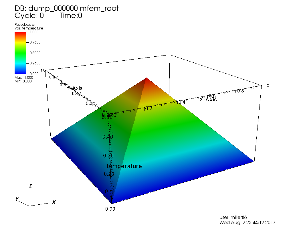
Here, all the runs solve a problem with an initial condition is a pyramid with value of 1 at the apex in the middle of the computational domain and zero on the boundaries as pictured in Figure 1.
| Figure 1 | Figure 2 |
|---|---|
 |
 |
The main loop of transient-heat.cpp is shown here…
304    // Perform time-integration
309    ode_solver->Init(oper);
310    double t = 0.0;
311    bool last_step = false;
312    for (int ti = 1; !last_step; ti++)
313    {
319       ode_solver->Step(u, t, dt);
320
327       u_gf.SetFromTrueDofs(u);
328
336       oper.SetParameters(u);
337       last_step = (t >= t_final - 1e-8*dt);
338    }
Later in this lesson, we’ll show the lines of code that permit the application great flexibility in how it employs SUNDIALS to handle time integration.
Getting Help
$ ./transient-heat --help
Usage: ./transient-heat [options] ...
Options:
   -h, --help
        Print this help message and exit.
   -d <int>, --dim <int>, current value: 2
        Number of dimensions in the problem (1 or 2).
   -r <int>, --refine <int>, current value: 0
        Number of times to refine the mesh uniformly.
   -o <int>, --order <int>, current value: 1
        Order (degree) of the finite elements.
   -ao <int>, --arkode-order <int>, current value: 4
        Order of the time integration scheme.
   -tf <double>, --t-final <double>, current value: 0.1
        Final time; start time is 0.
   -dt <double>, --time-step <double>, current value: 0.001
        When using a fixed step, time step size.
   -a <double>, --alpha <double>, current value: 0.2
        Alpha coefficient for conductivity: kappa + alpha*temperature
   -k <double>, --kappa <double>, current value: 0.5
        Kappa coefficient conductivity: kappa + alpha*temperature
   -art <double>, --arkode-reltol <double>, current value: 0.0001
        Relative tolerance for ARKODE time integration.
   -aat <double>, --arkode-abstol <double>, current value: 0.0001
        Absolute tolerance for ARKODE time integration.
   -adt, --adapt-time-step, -fdt, --fixed-time-step, current option: --fixed-time-step
        Flag whether or not to adapt the time step.
   -imp, --implicit, -exp, --explicit, current option: --explicit
        Implicit or Explicit ODE solution.
   -v, --visit, -nov, --no_visit, current option: --no_visit
        Enable dumping of visit files.
Note: This application may be used to solve the same equation used in
Lesson 1 by using command line options
-d 1 -alpha 0. The role of Lesson 1’s
is played by
here.
For all of the runs here, the application’s default behavior is to set
to 0.2 and
to 0.5.
Run 1: Explicit, Fixed  of 0.001
$ ./transient-heat -dt 0.001 --arkode-order 4 --explicit
Options used:
   --dim 2
   --refine 0
   --order 1
   --arkode-order 4
   --t-final 0.1
   --time-step 0.001
   --alpha 0.2
   --kappa 0.5
   --arkode-reltol 0.0001
   --arkode-abstol 0.0001
   --fixed-time-step
   --explicit
   --visit
Number of temperature unknowns: 289
Integrating the ODE ...
step 1, t = 0.001
ARKODE:
  num steps: 1, num evals: 7, num lin setups: 0, num nonlin sol iters: 0
  method order: 4, last dt: 0.001, next dt: 0.001
step 2, t = 0.002
ARKODE:
  num steps: 2, num evals: 13, num lin setups: 0, num nonlin sol iters: 0
  method order: 4, last dt: 0.001, next dt: 0.001
step 3, t = 0.003
ARKODE:
  num steps: 3, num evals: 19, num lin setups: 0, num nonlin sol iters: 0
  method order: 4, last dt: 0.001, next dt: 0.001
.
.
.
ARKODE:
  num steps: 97, num evals: 583, num lin setups: 0, num nonlin sol iters: 0
  method order: 4, last dt: 0.001, next dt: 0.001
step 98, t = 0.098
ARKODE:
  num steps: 98, num evals: 589, num lin setups: 0, num nonlin sol iters: 0
  method order: 4, last dt: 0.001, next dt: 0.001
step 99, t = 0.099
ARKODE:
  num steps: 99, num evals: 595, num lin setups: 0, num nonlin sol iters: 0
  method order: 4, last dt: 0.001, next dt: 0.001
step 100, t = 0.1
ARKODE:
  num steps: 100, num evals: 601, num lin setups: 0, num nonlin sol iters: 0
  method order: 4, last dt: 0.001, next dt: 0.001
Integer ops        = 1010644516
Floating point ops = 57427320
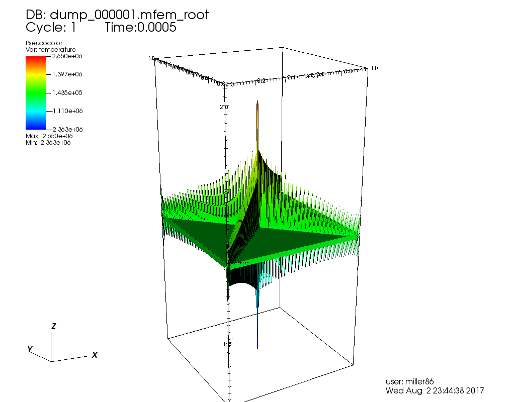
The first few time steps of this explicit algorithm are plotted below.
| Time Step 0 | Time Step 1 | Time Step 2 |
|---|---|---|
|
 |
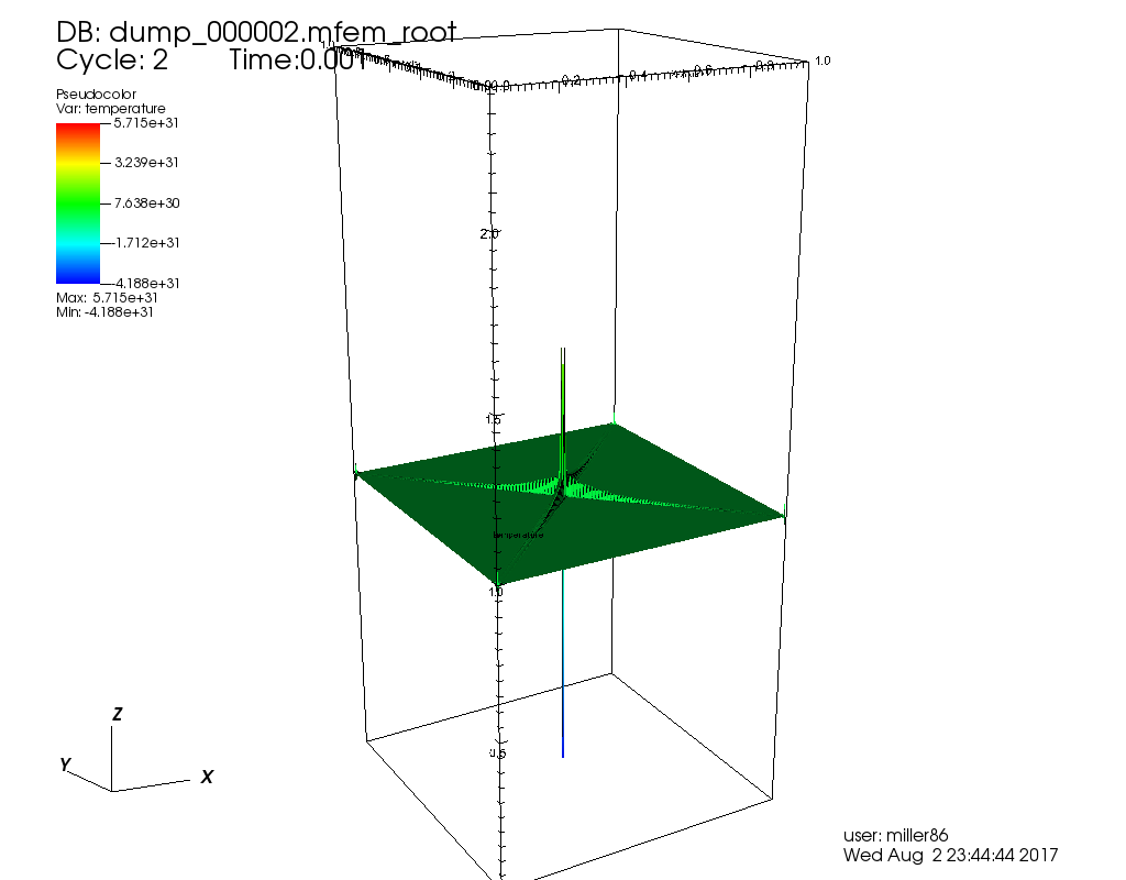 |
What do you think happened? (triple-click box below to reveal answer)
| The explicit algorithm is unstable for the specified timestep size. |
How can we make this explicit method work? (triple-click box below to reveal answer)
| We can shrink the timestep. |
Run 2: Explicit, Smaller of 0.0005
[mcmiller@cooleylogin1 ~/tmp]$ ./transient-heat -dt 0.0005 --arkode-order 4 --explicit
Options used:
   --dim 2
   --refine 0
   --order 1
   --arkode-order 4
   --t-final 0.1
   --time-step 0.0005
   --alpha 0.2
   --kappa 0.5
   --arkode-reltol 0.0001
   --arkode-abstol 0.0001
   --fixed-time-step
   --explicit
   --visit
Number of temperature unknowns: 289
Integrating the ODE ...
step 1, t = 0.0005
ARKODE:
  num steps: 1, num evals: 7, num lin setups: 0, num nonlin sol iters: 0
  method order: 4, last dt: 0.0005, next dt: 0.0005
step 2, t = 0.001
ARKODE:
  num steps: 2, num evals: 13, num lin setups: 0, num nonlin sol iters: 0
  method order: 4, last dt: 0.0005, next dt: 0.0005
step 3, t = 0.0015
ARKODE:
  num steps: 3, num evals: 19, num lin setups: 0, num nonlin sol iters: 0
  method order: 4, last dt: 0.0005, next dt: 0.0005
.
.
.
step 198, t = 0.099
ARKODE:
  num steps: 198, num evals: 1189, num lin setups: 0, num nonlin sol iters: 0
  method order: 4, last dt: 0.0005, next dt: 0.0005
step 199, t = 0.0995
ARKODE:
  num steps: 199, num evals: 1195, num lin setups: 0, num nonlin sol iters: 0
  method order: 4, last dt: 0.0005, next dt: 0.0005
step 200, t = 0.1
ARKODE:
  num steps: 200, num evals: 1201, num lin setups: 0, num nonlin sol iters: 0
  method order: 4, last dt: 0.0005, next dt: 0.0005
Integer ops        = 2330325813
Floating point ops = 181844398
| Time Step 7 | Time Step 32 | Time Step 100 |
|---|---|---|
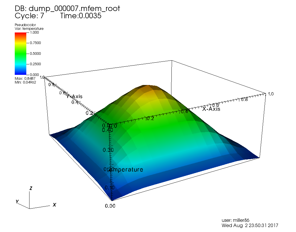 |
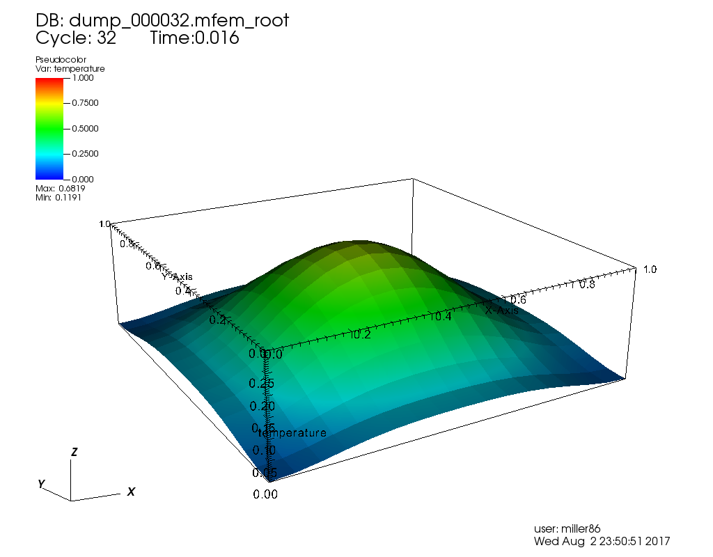 |
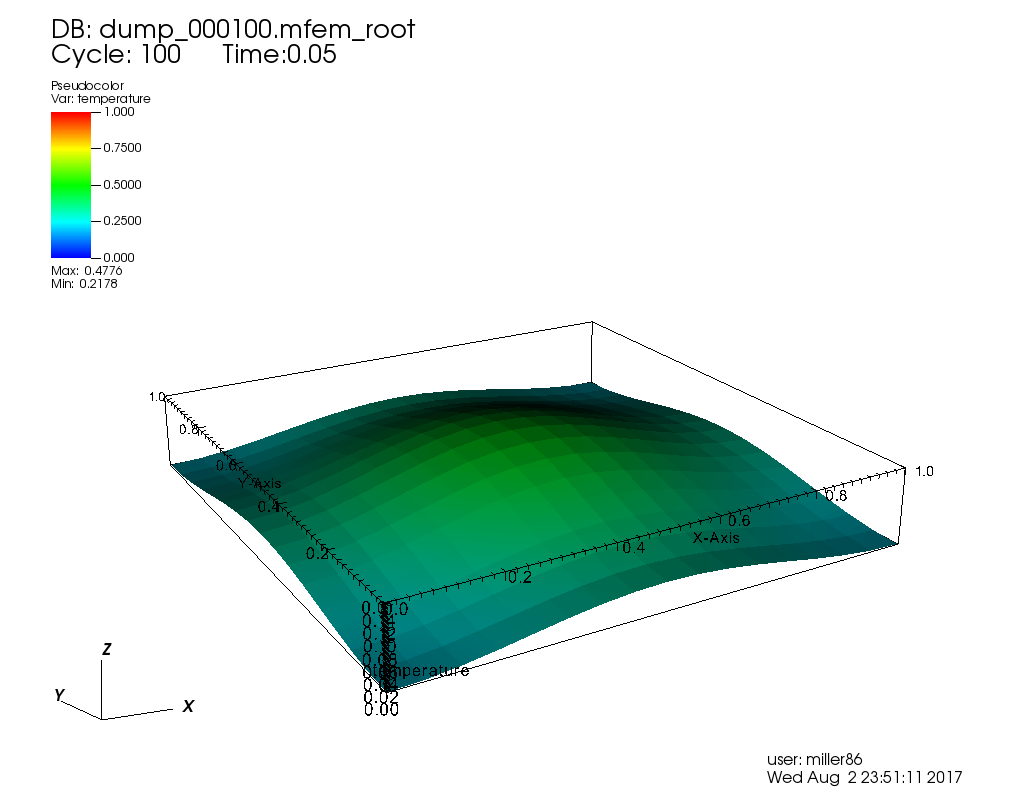 |
Run 3: Explicit, Adaptive Absolute and Relative Tolerance 1e-6
Now, we will switch to an adaptive time stepping method using the -adt
command-line option but keeping all other options the same.
[mcmiller@cooleylogin1 ~/tmp]$ ./transient-heat -adt --arkode-order 4 --arkode-abstol 1e-6 --arkode-reltol 1e-6 --explicit
Options used:
   --dim 2
   --refine 0
   --order 1
   --arkode-order 4
   --t-final 0.1
   --time-step 0.001
   --alpha 0.2
   --kappa 0.5
   --arkode-reltol 1e-06
   --arkode-abstol 1e-06
   --adapt-time-step
   --explicit
   --visit
Number of temperature unknowns: 289
Integrating the ODE ...
step 1, t = 1.3850325e-09
ARKODE:
  num steps: 1, num evals: 10, num lin setups: 0, num nonlin sol iters: 0
  method order: 4, last dt: 1.3850325e-09, next dt: 1.1404192e-07
step 2, t = 1.1542696e-07
ARKODE:
  num steps: 2, num evals: 16, num lin setups: 0, num nonlin sol iters: 0
  method order: 4, last dt: 1.1404192e-07, next dt: 1.8735665e-06
step 3, t = 1.9889934e-06
ARKODE:
  num steps: 3, num evals: 22, num lin setups: 0, num nonlin sol iters: 0
  method order: 4, last dt: 1.8735665e-06, next dt: 2.9257093e-05
.
.
.
step 134, t = 0.098921587
ARKODE:
  num steps: 134, num evals: 853, num lin setups: 0, num nonlin sol iters: 0
  method order: 4, last dt: 0.00078192401, next dt: 0.00078192401
step 135, t = 0.099703512
ARKODE:
  num steps: 135, num evals: 859, num lin setups: 0, num nonlin sol iters: 0
  method order: 4, last dt: 0.00078192401, next dt: 0.00078192401
step 136, t = 0.1
ARKODE:
  num steps: 136, num evals: 865, num lin setups: 0, num nonlin sol iters: 0
  method order: 4, last dt: 0.0002964885, next dt: 0.0002964885
Integer ops        = 2085145055
Floating point ops = 199642899
| Plot of |
|---|
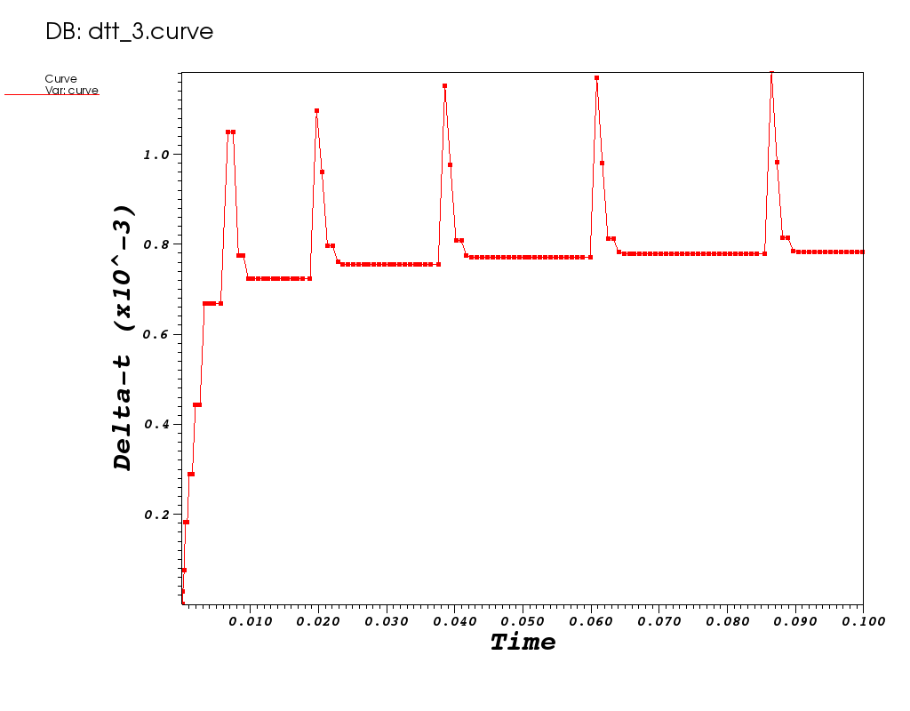 |
How many steps did this method take and how many flops?
| By adapting the timestep, we took only 136 steps to the solution at t=0.1. There are about 10% more flops required, however, in total. |
A plot of the time step size vs. time is shown above. Can you explain its shape?
| Recall the explicit method we are using here is unstable for dt=0.001 but is stable for dt=0.0005. The adaptive algorithm is attempting to adapt the timestep. It attemps step sizes outside of the regime of stability and may even get away with a few steps in that regime before having to shrink the timestep back down to maintain stability. Note the majority of timestep sizes used are between 0.0007 and 0.0008 which is just butting up against the timestep threshold of stability for this particular 4th order algorithm. |
Run 4: Implicit, Fixed at 0.001
Now, lets switch to an implicit method and see how that effects behavior of the numerical algorithms.
[mcmiller@cooleylogin1 ~/tmp]$ ./transient-heat -dt 0.001 --arkode-order 4 --implicit
Options used:
   --dim 2
   --refine 0
   --order 1
   --arkode-order 4
   --t-final 0.1
   --time-step 0.001
   --alpha 0.2
   --kappa 0.5
   --arkode-reltol 0.0001
   --arkode-abstol 0.0001
   --fixed-time-step
   --implicit
   --visit
Number of temperature unknowns: 289
Integrating the ODE ...
step 1, t = 0.001
ARKODE:
  num steps: 1, num evals: 0, num lin setups: 1, num nonlin sol iters: 10
  method order: 4, last dt: 0.001, next dt: 0.001
step 2, t = 0.002
ARKODE:
  num steps: 2, num evals: 0, num lin setups: 1, num nonlin sol iters: 16
  method order: 4, last dt: 0.001, next dt: 0.001
step 3, t = 0.003
ARKODE:
  num steps: 3, num evals: 0, num lin setups: 1, num nonlin sol iters: 21
  method order: 4, last dt: 0.001, next dt: 0.001
.
.
.
ARKODE:
  num steps: 97, num evals: 0, num lin setups: 5, num nonlin sol iters: 509
  method order: 4, last dt: 0.001, next dt: 0.001
step 98, t = 0.098
ARKODE:
  num steps: 98, num evals: 0, num lin setups: 5, num nonlin sol iters: 514
  method order: 4, last dt: 0.001, next dt: 0.001
step 99, t = 0.099
ARKODE:
  num steps: 99, num evals: 0, num lin setups: 5, num nonlin sol iters: 519
  method order: 4, last dt: 0.001, next dt: 0.001
step 100, t = 0.1
ARKODE:
  num steps: 100, num evals: 0, num lin setups: 5, num nonlin sol iters: 524
  method order: 4, last dt: 0.001, next dt: 0.001
Integer ops        = 2331254488
Floating point ops = 248347397
Take note of the number of non-linear solution iterations here, 524 and total flops 248347397.
How does the flop count in this implicit fixed time step method compare with the explicit fixed time step method?
| Well, at a dt=0.001, the explicit method failed due to stability issues. But, it suceeded with a dt=0.0005, which required twice as many steps to reach t=0.1 where the _implicit_ succeeds with dt=0.001 but still requires about 33% more flops due to the implicit solves needed on each step. The cost of the implicit method may be reduced by using looser tolerances if those are appropriate for the application needs. |
How is all the flexiblity demonstrated here possible?
| The lines of code below illustrate how the application is taking advantage of the SUNDIALS numerical package to affect various methods of solution. |
204    // Define the ARKODE solver used for time integration. Either implicit or explicit.
205    ODESolver *ode_solver = NULL;
206    ARKODESolver *arkode = NULL;
207    SundialsJacSolver sun_solver; // Used by the implicit ARKODE solver.
208    if (implicit)
209    {
210       arkode = new ARKODESolver(MPI_COMM_WORLD, ARKODESolver::IMPLICIT);
211       arkode->SetLinearSolver(sun_solver);
212    }
213    else
214    {
215       arkode = new ARKODESolver(MPI_COMM_WORLD, ARKODESolver::EXPLICIT);
216       //arkode->SetERKTableNum(FEHLBERG_13_7_8);
217    }
218    arkode->SetStepMode(ARK_ONE_STEP);
219    arkode->SetSStolerances(arkode_reltol, arkode_abstol);
220    arkode->SetOrder(arkode_order);
221    arkode->SetMaxStep(t_final / 2.0);
222    if (!adaptdt)
223    {
224       arkode->SetFixedStep(dt);
225    }
226    ode_solver = arkode;
Note lines 210/215 that select either implicit or _explicit method. Lines 220 sets the order of the method and line 224 sets a fixed time step whereas the default is an adaptive timestep.
Run 5: Implicit, Fixed at 0.001, 2nd Order
Here, we reduce the order of the time-integration from 4 to 2 and observe the behavior.
[mcmiller@cooleylogin1 ~/tmp]$ ./transient-heat -dt 0.001 --arkode-order 2 --implicit
Options used:
   --dim 2
   --refine 0
   --order 1
   --arkode-order 2
   --t-final 0.1
   --time-step 0.001
   --alpha 0.2
   --kappa 0.5
   --arkode-reltol 0.0001
   --arkode-abstol 0.0001
   --fixed-time-step
   --implicit
   --visit
Number of temperature unknowns: 289
Integrating the ODE ...
step 1, t = 0.001
ARKODE:
  num steps: 1, num evals: 0, num lin setups: 1, num nonlin sol iters: 4
  method order: 2, last dt: 0.001, next dt: 0.001
step 2, t = 0.002
ARKODE:
  num steps: 2, num evals: 0, num lin setups: 1, num nonlin sol iters: 8
  method order: 2, last dt: 0.001, next dt: 0.001
step 3, t = 0.003
ARKODE:
  num steps: 3, num evals: 0, num lin setups: 1, num nonlin sol iters: 11
  method order: 2, last dt: 0.001, next dt: 0.001
step 4, t = 0.004
.
.
.
step 98, t = 0.098
ARKODE:
  num steps: 98, num evals: 0, num lin setups: 5, num nonlin sol iters: 220
  method order: 2, last dt: 0.001, next dt: 0.001
step 99, t = 0.099
ARKODE:
  num steps: 99, num evals: 0, num lin setups: 5, num nonlin sol iters: 222
  method order: 2, last dt: 0.001, next dt: 0.001
step 100, t = 0.1
ARKODE:
  num steps: 100, num evals: 0, num lin setups: 5, num nonlin sol iters: 224
  method order: 2, last dt: 0.001, next dt: 0.001
Integer ops        = 1482885073
Floating point ops = 119982846
This second order method succeeds in about 1/2 the number of flops and nonlinear iterations. Why?
| High order time-integration is not always required or the best approach. By paying attention to the time-integration order requirements of your particular application, you can indeed reduce flop counts required. |
Run 6: Implicit, Adaptive , Tolerances 1e-6, 4th Order
In this run, we’ll combine both the advantages of an implicit algorithm and an adaptive time step.
[mcmiller@cooleylogin1 ~/tmp]$ ./transient-heat -adt --arkode-order 4 --arkode-abstol 1e-6 --arkode-reltol 1e-6 --implicit
Options used:
   --dim 2
   --refine 0
   --order 1
   --arkode-order 4
   --t-final 0.1
   --time-step 0.001
   --alpha 0.2
   --kappa 0.5
   --arkode-reltol 1e-06
   --arkode-abstol 1e-06
   --adapt-time-step
   --implicit
   --visit
Number of temperature unknowns: 289
Integrating the ODE ...
step 1, t = 1.3850325e-09
ARKODE:
  num steps: 1, num evals: 0, num lin setups: 1, num nonlin sol iters: 5
  method order: 4, last dt: 1.3850325e-09, next dt: 1.1404192e-07
step 2, t = 1.1542696e-07
ARKODE:
  num steps: 2, num evals: 0, num lin setups: 2, num nonlin sol iters: 10
  method order: 4, last dt: 1.1404192e-07, next dt: 1.8735665e-06
step 3, t = 1.9889934e-06
ARKODE:
  num steps: 3, num evals: 0, num lin setups: 3, num nonlin sol iters: 17
  method order: 4, last dt: 1.8735665e-06, next dt: 3.7471329e-05
.
.
.
ARKODE:
  num steps: 24, num evals: 0, num lin setups: 14, num nonlin sol iters: 189
  method order: 4, last dt: 0.012499762, next dt: 0.019204807
step 25, t = 0.09505614
ARKODE:
  num steps: 25, num evals: 0, num lin setups: 15, num nonlin sol iters: 199
  method order: 4, last dt: 0.019204807, next dt: 0.019204807
step 26, t = 0.1
ARKODE:
  num steps: 26, num evals: 0, num lin setups: 16, num nonlin sol iters: 209
  method order: 4, last dt: 0.0049438602, next dt: 0.0049438602
Integer ops        = 1009761594
Floating point ops = 115569416
| Plot of |
|---|
 |
How many steps and flops does it take to reach t=0.1?
| The algorithm reaches t=0.1 in 26 steps but about the same number of flops. |
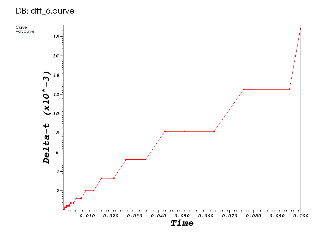
A plot of dt vs. time is shown above. Why is it able to continue increasing dt?
| This is using a stable implicit method. As time increases, the solution changes more slowly allow the time-integration to continue to increase. Contrast this with adaptive time stepping for the explicit case where it would try to increase the step size and then constantly have to back up to maintain stability. |
Run 7: Implicit, Adaptive , Tolerances 1e-6, 2nd Order
Here, like Run 5, we compare to the preceding run with a 2nd order method.
[mcmiller@cooleylogin1 ~/tmp]$ ./transient-heat -adt --arkode-order 2 --arkode-abstol 1e-6 --arkode-reltol 1e-6 --implicit
Options used:
   --dim 2
   --refine 0
   --order 1
   --arkode-order 2
   --t-final 0.1
   --time-step 0.001
   --alpha 0.2
   --kappa 0.5
   --arkode-reltol 1e-06
   --arkode-abstol 1e-06
   --adapt-time-step
   --implicit
   --visit
Number of temperature unknowns: 289
Integrating the ODE ...
step 1, t = 1.3850325e-09
ARKODE:
  num steps: 1, num evals: 0, num lin setups: 1, num nonlin sol iters: 2
  method order: 2, last dt: 1.3850325e-09, next dt: 1.3850325e-05
step 2, t = 1.385171e-05
ARKODE:
  num steps: 2, num evals: 0, num lin setups: 2, num nonlin sol iters: 5
  method order: 2, last dt: 1.3850325e-05, next dt: 1.3850325e-06
step 3, t = 1.5236743e-05
ARKODE:
  num steps: 3, num evals: 0, num lin setups: 3, num nonlin sol iters: 8
  method order: 2, last dt: 1.3850325e-06, next dt: 2.770065e-05
.
.
.
ARKODE:
  num steps: 125, num evals: 0, num lin setups: 18, num nonlin sol iters: 313
  method order: 2, last dt: 0.0029289748, next dt: 0.0028752935
step 126, t = 0.095340247
ARKODE:
  num steps: 126, num evals: 0, num lin setups: 18, num nonlin sol iters: 316
  method order: 2, last dt: 0.0028752935, next dt: 0.0028752935
step 127, t = 0.09821554
ARKODE:
  num steps: 127, num evals: 0, num lin setups: 18, num nonlin sol iters: 319
  method order: 2, last dt: 0.0028752935, next dt: 0.0028752935
step 128, t = 0.1
ARKODE:
  num steps: 128, num evals: 0, num lin setups: 19, num nonlin sol iters: 323
  method order: 2, last dt: 0.0017844596, next dt: 0.0017844596
Integer ops        = 2279562091
Floating point ops = 218387843
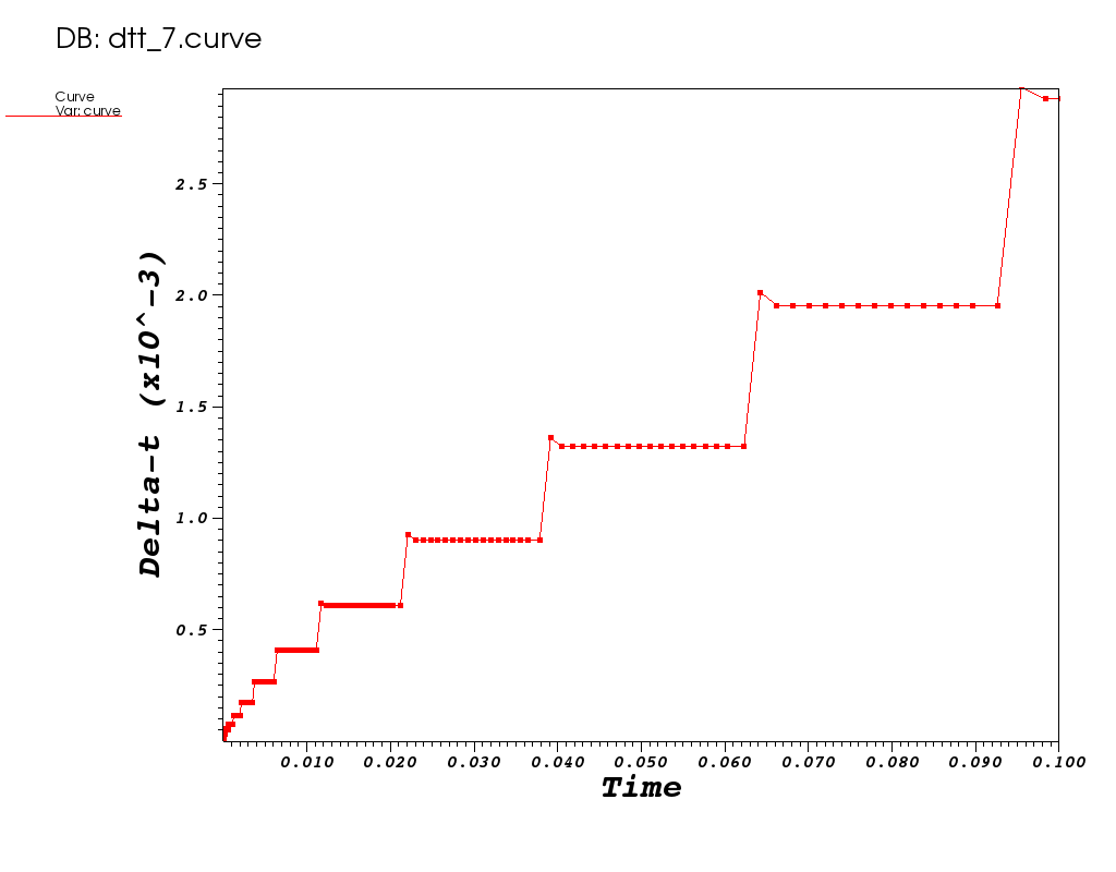
Why does the algorithm take more steps to reach t=0.1?
| The lower order (2 as compared to 4) we are using here means the algorithm is unable to maintain the desired tolerances at larger step sizes. In general, the step sizes are smaller for a lower order method so more steps are required to reach t=0.1 |
| Plot of |
|---|
 |
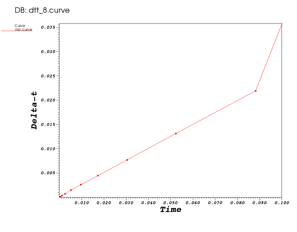
Run 8: Implicit, Adaptive , Tolerances 1e-6, 5th Order
Here, for a final comparison, we increase to order 5 and observe the impact.
[mcmiller@cooleylogin1 ~/tmp]$ ./transient-heat -adt --arkode-order 5 --arkode-abstol 1e-6 --arkode-reltol 1e-6 --implicit
Options used:
   --dim 2
   --refine 0
   --order 1
   --arkode-order 5
   --t-final 0.1
   --time-step 0.001
   --alpha 0.2
   --kappa 0.5
   --arkode-reltol 1e-06
   --arkode-abstol 1e-06
   --adapt-time-step
   --implicit
   --visit
Number of temperature unknowns: 289
Integrating the ODE ...
step 1, t = 1.3850325e-09
ARKODE:
  num steps: 1, num evals: 0, num lin setups: 1, num nonlin sol iters: 7
  method order: 5, last dt: 1.3850325e-09, next dt: 3.7474099e-08
step 2, t = 3.8859132e-08
ARKODE:
  num steps: 2, num evals: 0, num lin setups: 2, num nonlin sol iters: 14
  method order: 5, last dt: 3.7474099e-08, next dt: 3.0269304e-07
step 3, t = 3.4155217e-07
ARKODE:
  num steps: 3, num evals: 0, num lin setups: 3, num nonlin sol iters: 22
  method order: 5, last dt: 3.0269304e-07, next dt: 4.3478412e-06
step 4, t = 4.6893933e-06
.
.
.
ARKODE:
  num steps: 12, num evals: 0, num lin setups: 12, num nonlin sol iters: 140
  method order: 5, last dt: 0.013108521, next dt: 0.021859715
step 13, t = 0.052228858
ARKODE:
  num steps: 13, num evals: 0, num lin setups: 13, num nonlin sol iters: 154
  method order: 5, last dt: 0.021859715, next dt: 0.035793708
step 14, t = 0.088022566
ARKODE:
  num steps: 14, num evals: 0, num lin setups: 14, num nonlin sol iters: 168
  method order: 5, last dt: 0.035793708, next dt: 0.05
step 15, t = 0.1
ARKODE:
  num steps: 15, num evals: 0, num lin setups: 15, num nonlin sol iters: 181
  method order: 5, last dt: 0.011977434, next dt: 0.011977434
Integer ops        = 893073353
Floating point ops = 108013134
A comparison of the three, preceding implicit, adaptive methods at order 4, 2 and 5 is shown below
Plot of vs t for 3 succeeding implicit, adaptive runs
| O=2, N=128, F=218387843 | O=4, N=26, F=115569416 | O=5, N=15, F=108013134 |
|---|---|---|
| N=Nn, F=Fn (normalized) | N=0.2 Nn, F=0.5 Fn | N=0.12 Nn, F=0.5 Fn |
|
|
 |
Out-Brief
We have used MFEM as a demonstration vehicle for illustrating the value in robust, time integration methods in numerical algorithms. In particular, we have used the SUNDIALS suite of solvers to compare and contrast both the effects of adaptive time stepping as well as the role the order of the time integration plays in time to solution and number of time steps in the adaptive case. In addition, we have demonstrated the ability of implicit methods to run at higher time steps than explicit and also demonstrated the cost of nonlinear solvers in implicit approaches.
The use of adaptation here was confined to discretzation of time. Other lessons here demonstrate the advantages adaptation can play in the discretization of space.
Other lessons will demonstrate some of the options for nonlinear and linear solvers needed for implicit integration approaches.
Finally, it is worth reminding the learner that the application demonstrated here can be run on 1, 2 and 3 dimensional meshes and in scalable, parallel settings on on meshes of extremely high spatial resolution if so desired. The learner is encouraged to play around with various command-line options to affect various scenarios.
Further Reading
Users guides for CVODE, ARKode, and IDA