A Block Structured Adaptive Mesh Refinement Framework

Meshing and Discretization with AMReX

Not your grandmother's AMR...!

At a Glance

Questions	Objectives	Key Points
What can I do with AMReX?	Understand that “AMR” means more than just “traditional AMR”	AMR + EB + Particles
How do I get started?	Understand easy set-up	It’s not hard to get started
How do I visualize AMR results?	Use Visit and Paraview for AMReX vis	Visualization tools exist for AMR data.

Example: Multi-Level Scalar Advection

What Features Are We Using

Mesh data
Dynamic AMR with subcycling

The Problem

Consider a drop of dye (we’ll define \(\phi\) to be the concentration of dye) in a thin incompressible fluid that is spinning clock-wise then counter-clockwise with a prescribed motion. We consider the dye to be a passive tracer that is advected by the fluid velocity. The fluid is thin enough that we can model this as two-dimensional motion.

In other words, we want to solve for \(\phi(x,y,t)\) by evolving \[\frac{\partial \phi}{\partial t} + \nabla \cdot (\bf{u} \phi) = 0\]

in time (\(t\)), where the velocity \({\bf{u}} = (u,v)\) is a divergence-free field computed by defining \[\psi(i,j) = \sin^2(\pi x) \sin^2(\pi y) \cos (\pi t / 2) / \pi\]

and defining \[u = -\frac{\partial \psi}{\partial y}, v = \frac{\partial \psi}{\partial x}.\]

In this example we’ll be using AMR to resolve the scalar field since the location of the dye is what we care most about.

To update the solution at each level, we call an advance routine that computes fluxes (\({\bf u} \phi\)) on each face, and differences the fluxes to create the update to phi. In this example the update happens in a Fortran subroutine that operates on one grid of data at a time. Here “lo()” and “hi()” are the bounds of the one grid we are operating on, not of the entire domain.

Knowing how to synchronize the solution at coarse/fine boundaries is essential in an AMR algorithm; here having the algorithm written in flux form allows straightforward “refluxing” at coarse-fine interfaces.

At each level:

  ! Do a conservative update
  do    j = lo(2),hi(2)
     do i = lo(1),hi(1)
        phi_new(i,j) = phi_old(i,j) + &
             ( (flxx(i,j) - flxx(i+1,j)) * dtdx(1) &
             + (flxy(i,j) - flxy(i,j+1)) * dtdx(2) )
     enddo
  enddo

If “timeStep(lev,…)” is the routine that creates the fluxes and advances the solution at level “lev”, then the subcycling in time algorithm looks like:

    if (lev < finest_level)
    {
        // recursive call for next-finer level
        for (int i = 1; i <= nsubsteps[lev+1]; ++i)
        {
            timeStep(lev+1, time+(i-1)*dt[lev+1], i);
        }

        if (do_reflux)
        {
            // update lev based on coarse-fine flux mismatch
            flux_reg[lev+1]->Reflux(*phi_new[lev], 1.0, 0, 0, phi_new[lev]->nComp(), geom[lev]);
        }

        AverageDownTo(lev); // average lev+1 down to lev
    }

Note that if “nsubsteps” is greater than 1, we are “subcycling” in time, ie using a smaller dt at the finer levels.

Running the Code

cd HandsOnLessons/amrex/AMReX_Amr_Advection

In this directory you’ll see

main2d.gnu.MPI.ex -- the executable -- this has been built with MPI 

inputs -- an inputs file

To run in serial,

./main2d.gnu.MPI.ex inputs

To run in parallel, for example on 4 ranks:

mpirun -n 4 ./main2d.gnu.MPI.ex inputs

The following parameters can be set at run-time – these are currently set in the inputs file but you can also set them on the command line.

amr.max_time       =  2.0                # the final time (if max_time < max_steps * time_step)

amr.max_steps      = 1000000             # the maximum number of steps (if max_steps * time_step < max_time))

amr.n_cell         =  64   64   64       # number of cells at the coarsest AMR level in each coordinate direction

amr. max_grid_size = 32                  # the maximum number of cells in any direction in a single grid

amr.plot_int       = 10                  # frequency of writing plotfiles

adv.cfl            = 0.7                 # cfl number to be used for computing the time step

adv.phierr = 1.01  1.1  1.5              # regridding criteria  at each level

The base grid here is a square of 64 x 64 cells, made up of 4 subgrids each of size 32x32 cells.
The problem is periodic in both the x-direction and y-direction.

We have hard-wired the code here to refine based on the magnitude of \(\phi\). Here we set the threshold level by level. If \(\phi > 1.01\) then we want to refine at least once; if \(\phi > 1.1\) we want to resolve \(\phi\) with two levels of refinement, and if \(\phi > 1.5\) we want even more refinement.

Visualizing the Results

Sample solution

After you run the code you will have a series of plotfiles. To visualize these we will use the VisIt package.

To use the VisIt python script, simply do the following to generate amr_advection.mp4:

$ make movie

(You will need +ffmpeg in your .soft.cooley file, and this assumes that python2 is the Python 2 interpreter. If python is the Python 2 interpreter, you can do make movie PYTHON2=python).

To do the same thing with the VisIt client-server interface to Cooley, here are the instructions:

On Cooley, in the tutorial directory, run the command, "ls -1 plt*/Header | tee movie.visit"
Start VisIt and connect to Cooley. 
File --> Open file ... go to Cooley and select movie.visit 
In the Plots pane, go to Add/Pseudocolor and select the field phi
In the Plots pane, go to Add/Subset and select "patches"
Open the options for the "patches" subset object and select "Wireframe"
Go to Controls/Animation and select "Cache animation ..."
Press the "Play" button

Topics to Explore

What happens as you change the max grid size for decomposition?
What happens as you change the refinement criteria (i.e. use different values of \(\phi\))? (You can edit these in inputs)
How does runtime scale with number of processors? To give the problem sufficient work for 4 processors, run it as, e.g:

mpiexec -n 4 ./main2d.gnu.MPI.ex inputs amr.n_cell=256 256 amr.max_level=3 max_step=50

Example: “Off to the Races”

What Features Are We Using

Mesh data with EB
Linear solvers (multigrid)
Tracer Particles

The Problem

Challenge:

Imagine incompressible flow in a channel from left to right. The inflow velocity on the left is \(u = 1\).

If there are no obstacles in the channel, the fluid will flow with speed 1 from left to right.

If you place obstacles in the channel, the fluid must flow around them.

Suppose your goal is to accelerate the fluid so that a tracer released near the inflow reaches the right side as fast as possible.

You are given nine cylinders that you can place (or not) at specified locations.

You can use particles released near the inflow to measure the fastest configuration.

How many cylinders should you use, and where should you put them?

Running the code

cd HandsOnLessons/amrex/AMReX_EB_MacProj

Sample solution

In this directory you’ll see

main3d.ex -- the executable -- this has been built with MPI 

inputs_3d -- domain size, size of grids, how many time steps, which obstacles...

initial_particles_3d -- initial particle locations  (this name is given in the inputs_3d file)

To run in serial,

./main3d.ex inputs_3d

To run in parallel, for example on 4 ranks:

mpirun -n 4 ./main3d.ex inputs_3d

The following parameters can be set at run-time – these are currently set in the inputs_3d file.

n_cell = 128                             # number of cells in x-direction; we double this in the y-direction
max_grid_size = 64                       # the maximum number of cells in any direction in a single grid

plot_int = 10                            # frequency of writing plotfiles

particle_file = initial_particles_3d     # name of file where we specify the input positions of the particles

time_step = 0.001                        # we advance the particles with a fixed time step of this size

max_time = 10.0                          # the final time (if max_time < max_steps * time_step)

max_steps = 10000                        # the maximum number of steps (if max_steps * time_step < max_time))

obstacles = 0 1 2 3 4 5 6 7 8            # this is how we choose which obstacles to include

We define the cylinders with this numbering scheme

Numbering

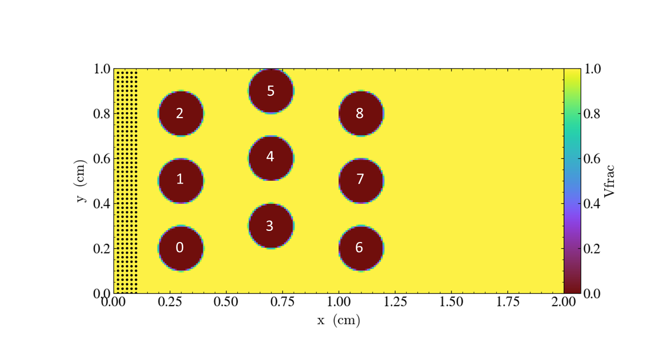
You can also set the parameters on the command line; for example,

mpirun -n 4 ./main3d.ex inputs_3d obstacles = 1 3 4 5 6 8

will run the problem with only six obstacles

The output from your run should look something like this:

********************************************************************
 You specified 9 objects in the domain: 0 1 2 3 4 5 6 7 8
 ********************************************************************

********************************************************************
 First let's project the initial velocity to find
   the flow field around the obstacles ...
********************************************************************


********************************************************************
 Done!  Now let's advect the particles ...
********************************************************************

Timestep 0, Time = 0.001 and leading particle now at 0.101179325
Timestep 100, Time = 0.101 and leading particle now at 0.2444506795
Timestep 200, Time = 0.201 and leading particle now at 0.4330191808
Timestep 300, Time = 0.301 and leading particle now at 0.5611955983
Timestep 400, Time = 0.401 and leading particle now at 0.7422046938
Timestep 500, Time = 0.501 and leading particle now at 0.8955689091
Timestep 600, Time = 0.601 and leading particle now at 1.044585496
Timestep 700, Time = 0.701 and leading particle now at 1.225885881
Timestep 800, Time = 0.801 and leading particle now at 1.34851225
Timestep 900, Time = 0.901 and leading particle now at 1.45538891
Timestep 1000, Time = 1.001 and leading particle now at 1.558181566
Timestep 1100, Time = 1.101 and leading particle now at 1.659474158
Timestep 1200, Time = 1.201 and leading particle now at 1.760129699
Timestep 1300, Time = 1.301 and leading particle now at 1.860489498
Timestep 1400, Time = 1.401 and leading particle now at 1.960718531

********************************************************************
We have a winner...and the winning time is 1.431
********************************************************************

Note that if you want to figure out which is the fastest configuration, you’ll need to run the code multiple times with different configurations and compare the “winning times.” This is a good example of how we often don’t run the simulation code in a “one and done” mode – the simulation is often only one component of a science investigation or design process.

Visualizing the Results

We’ll use Paraview to visualize the results for this example.

To use the Paraview python script, simply do:

$ make movie

(You will need +ffmpeg in your .soft.cooley file)

To do the same thing with the ParaView client-server interface to Cooley, see the note below on how to set up the client-server interface for this tutorial.

There are three types of data from the simulation that we want to load:

the EB representation of the cylinders
the mesh data, which includes the velocity field and the processor ID
the particle motion

Because the EB data and mesh data don’t change, we load these separately from the particles.

Instructions to visualize the EB representation of the cylinders:

Start paraview
File --> Open ... select "eb.pvtp" (highlight it then click OK) 
Click green Apply button 

You should see cylinders with their axes in the z-direction.

Now to add the mesh field:

File --> Open ... make sure you are in the "AMReX_EB_MacProj" directory and double click on "plt.."
In the "Files of type:" window at the bottom select "All Files(*)"
Now highlight "Header" and click OK
You now have to select "VisitBoxlib3DReader" from the drop-down menu titled "Open Data With..." -- then click OK
 Click green Apply button 

This will display an outline of the grids (boxes)

With "Header" highlighted in the "Pipeline Browser" menu,
   click on "proc" and "vel" in the "Cell Arrays" menu 
Click green Apply button
Click on the "slice" icon -- three to the right of the calculator.
   This will create "Slice 1" in the Pipeline Browser which will be highlighted.
Click on "Z Normal"
Unclick the "Show Plane" button
Click green Apply button
Change the drop-down menu option (above the calculator row) from "vtkBlockColors" to "vel"
(We could also color the grid by "proc" -- the integer id of the processor owning that grid.)

Now to load the particles:

1. File --> Open ... make sure you are in the "AMReX_EB_MacProj" directory and highlight "plt.." 
   then click OK
2. With "plt0*" highlighted in the Pipeline Browser menu, click green Apply button
3. Click the "glyph" button (6 to the right of the calculator)
4. Under "Glyph Source" 
   * select "Sphere" instead of "Arrow"
   * set "Radius" to 0.01
6. Under "Scale" (down below "Glyph Source") set "Scale Factor" to 1 
7. Under "Masking" (down below "Scale") change "Glyph Mode" from "Uniform Spatial Distribution"
   to "All Points" 
8.  Click green Apply button 

You are now ready to play the movie! See the “VCR-like” controls at the top. Click the play button.

For fun: if you want to color the particles, make sure “Glyph1” is highlighted, then change the drop-down menu option (above the calculator row) from “vtkBlockColors” to “cpu” – if you have run with 4 processes then you will see the particles displayed with different colors.

Also note – if you want to clean up your run directory before doing another run, you can type “make pltclean” to remove the plt* and *.png files.

Example: AMReX-Pachinko

What Features Are We Using

EB for obstacles
Particle-obstacle and particle-wall collisions

The Problem

Have you ever played pachinko?

A pachinko machine is like a vertical pinball machine.

Balls are released at the top of the “playing field”, and bounce off obstacles as they fall.

The object of the game is to “capture” as many balls as possible.

In the AMReX-Pachinko game you can release as many particles as you like at the top of the domain, and the balls will freeze when they hit the bottom so you can see where they landed.

Your goal here is to see if you can cover the floor of the pachinko machine.

(Note that this is not completely realistic – the balls here don’t feel each other so they can overlap.)

Running the Code

cd HandsOnLessons/amrex/AMReX_EB_Pachinko

In this directory you’ll see

main3d.ex            -- the executable -- this has been built with MPI 

inputs_3d            -- domain size, size of grids, how many time steps, which obstacles...

initial_particles_3d -- initial particle locations  (this name is given in the inputs_3d file)

In this example there is no fluid (or other variable) stored on the mesh but we still sort the particles according to our spatial decomposition of the domain. If we run in parallel with 4 processors, we see the domain decomposition below – this results from using a z-order space-filling curve with the number of cells per grid as the cost function.

Sample solution

For now we freeze the obstacles (although if you look in the code it’s not hard to figure out how to change them!) but we can change the initial particle locations at run-time by editing the initial_particles_3d file.

To run in serial,

./main3d.ex inputs_3d

To run in parallel, for example on 4 ranks:

mpirun -n 4 ./main3d.ex inputs_3d

The following parameters can be set at run-time – these are currently set in the inputs_3d file. In this specific example we use only 4 cells in the z-direction regardless of n_cell.

n_cell = 125                          # number of cells in x-direction; we double this in the y-direction
max_grid_size = 25                    # the maximum number of cells in any direction in a single grid

plot_int = 10                         # frequency of writing plotfiles

particle_file = initial_particles_3d  # name of file where we specify the input positions of the particles

time_step = 0.001                     # we take a fixed time step of this size

max_time  = 3.0                       # the final time (if max_time < max_steps * time_step)
max_steps = 100000                    # the maximum number of steps (if max_steps * time_step < max_time))

You can also set values on the command line; for example,

mpirun -n 4 ./main3d.ex inputs_3d particle_file=my_file

will read the particles from a file called “my_file”

The output from your run should look something like this:

********************************************************************
 Let's advect the particles ...
   We'll print a dot every 10 time steps.
********************************************************************

.............................................................................................................................................................................................................................................................................................................

********************************************************************
We've finished moving the particles to time 3
That took 1.145916707 seconds.
********************************************************************

Visualizing the Results

Again we’ll use Paraview to visualize the results.

As before, to use the Paraview python script, simply do:

$ make movie

(You will need +ffmpeg in your .soft.cooley file)

To do the same thing with the ParaView client-server interface to Cooley, see the note below on how to set up the client-server interface for this tutorial.

Remember there are three types of data from the simulation that we want to load:

the EB representation of the cylinders
the mesh data, which includes just the processor ID for each grid
the particle motion

Because the EB data and mesh data don’t change, we load these separately from the particles.

Instructions to visualize the EB representation of the cylinders:

Start paraview
File --> Open ... select "eb.pvtp" (highlight it then click OK) 
Click green Apply button 

You should see cylinders with their axes in the z-direction.

Now to add the mesh field:

File --> Open ... make sure you are in the "AMReX_EB_Pachinko" directory and double click on "plt.."
In the "Files of type:" window at the bottom select "All Files(*)"
Now highlight "Header" and click OK
You now have to select "VisitBoxlib3DReader" from the drop-down menu titled "Open Data With..." -- then click OK
 Click green Apply button 

This will display an outline of the grids (boxes)

With "Header" highlighted in the "Pipeline Browser" menu,
   click on "proc" in the "Cell Arrays" menu 
Click green Apply button
Click on the "slice" icon -- three to the right of the calculator.
   This will create "Slice 1" in the Pipeline Browser which will be highlighted.
Click on "Z Normal"
Unclick the "Show Plane" button
Click green Apply button
Change the drop-down menu option (above the calculator row) from "vtkBlockColors" to "proc"
(We could also color the grid by "proc" -- the integer id of the processor owning that grid.)

Now to load the particles:

1. File --> Open ... make sure you are in the "AMReX_EB_Pachinko" directory and highlight "plt.." 
   then click OK
2. With "plt0*" highlighted in the Pipeline Browser menu, click green Apply button
3. Click the "glyph" button (6 to the right of the calculator)
4. Under "Glyph Source" 
   * select "Sphere" instead of "Arrow"
   * set "Radius" to 0.02 (or whatever you have set the particle_radius to in the inputs file
                           if you changed it)   
6. Under "Scale" (down below "Glyph Source") set "Scale Factor" to 1 
7. Under "Masking" (down below "Scale") change "Glyph Mode" from "Uniform Spatial Distribution"
   to "All Points" 
8. Click green Apply button 

You are now ready to play the movie! See the “VCR-like” controls at the top. Click the play button.

Also note – if you want to clean up your run directory before doing another run, you can type “make pltclean” to remove the plt* and *.png files.

Follow-up Questions

Why might it be important to have n_cell be a power of 2 in the “Race” example but not in the “Pachinko” example?
- In the “Race” example we use multigrid to solve for the flow field.
How different is the Pachinko code itself for 2D vs 3D?
- Not very! Search for the test on AMREX_SPACEDIM in the source files to see how few lines are different.
How could I make the parallel decomposition in the Pachinko example load balance the particle work?
- Use a cost function based on number of particles instead of number of grid cells.

Suggested Evening Activities

In the “AMR 101” example,
- what quantities could I choose as refinement criteria besides the magnitude of phi?
- what factors besides the refinement criteria define the size and shape of the grids? ( Hint: you might want to read this first: https://amrex-codes.github.io/amrex/docs_html/GridCreation.html )
In the “Off to the Races” example,
- what is the configuration of obstacles in which the first particle reaches the end-line in the shortest time?
- does making the grid finer make the particles not get “stuck” on the obstacles?
- would a different linear solver be faster? ( Hint: try adding “use_hypre = 1” to the inputs_3d file )
In the Pachinko example,
- how well can I control the final distribution of particles from the initial particle positions?
- if I made the number of grids in the domain be different, how would that change the domain decomposition?
- how could I modify the code to make the particles bounce off each other as well? Does AMReX have a way of doing that?

Starting the ParaView Server on Cooley

To work with AMReX plotfiles locally you can use ParaView 5.6.1 with the instructions above.

On Cooley, to use ParaView 5.6.1 in client-server mode with AMReX plotfiles, we will need to start the ParaView server from the following path:

$ cd /projects/ATPESC2019/MathPackagesTraining/ParaView-5.6.1-MPI-Linux-64bit/bin
$ mpiexec -f $COBALT_NODEFILE -np 1 ./pvserver --server-port=8000

After the ParaView server starts, it will report which node and port it is listening on.

Waiting for client...
Connection URL: cs://cc054:8000
Accepting connection(s): cc054:8000

You can then connect to this ParaView server from your local ParaView 5.6.1 client using the Manual/Forward directions here

Back to all HandsOnLessons

Back to all ATPESC 2019 Lessons

At a Glance

Example: Multi-Level Scalar Advection

What Features Are We Using

The Problem

Running the Code

Visualizing the Results

Topics to Explore

Example: “Off to the Races”

What Features Are We Using

The Problem

Running the code

Visualizing the Results

Example: AMReX-Pachinko

What Features Are We Using

The Problem

Running the Code

Visualizing the Results

Follow-up Questions

Suggested Evening Activities

Further Reading

Starting the ParaView Server on Cooley