Role and Impact of Time Integrators in Solution Accuracy and Computational Efficiency
Time Integration and Nonlinear Solvers with SUNDIALS
At a glance
| Questions | Objectives | Key Points |
| How do explicit, implicit or IMEX methods impact step size? | Compare methods at step sizes near the stability limit. | Choose time integration method to match the problem. |
| What is the impact of an adaptive technique? | Compare fixed and adaptive techniques. | Adaptive techniques can be robust reliable and reduce computational cost. |
| How does integration order impact cost? | Observe impact of order on time to solution and number of steps. | Changing integration order is simple allowing optimization for a given problem. |
| How does the nonlinear solver affect robustness/scalability? | Compare different solvers with implicit and IMEX methods. | Some methods require more work but are more robust and scalable. |
| What is the role and benefit of preconditioning? | Compare integration methods with and without preconditioning. | Preconditioning is critical for scalability. |
Note: To begin this lesson…
cd HandsOnLessons/time_integrators/sundials
source source_cooley_plotfile_tools.sh
(note: you should be able to recompile these executables with a simple make)
Also, if you do not already have the anaconda3-4.0.0 SoftEnv module loaded, please do so now,
soft add +anaconda3-4.0.0
The problem being solved
In this problem, we model the transport of a pollutant that has been released into a flow in a two dimensional domain. We want to determine both where the pollutant goes, and when it has diffused sufficiently to be of no further harm.
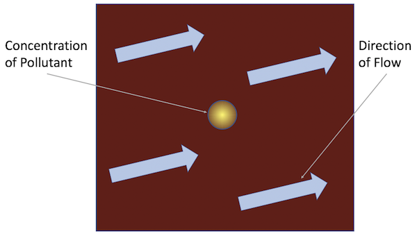
This is an example of a scalar-valued advection-diffusion problem for chemical transport. The governing equation is: \[\frac{\partial u}{\partial t} + \vec{a} \cdot \nabla u - \nabla \cdot ( D \nabla u ) = 0\]
where \(u = u(t,x,y)\) is the chemical concentration, \(\vec{a}\) is the advection vector, \(D\) is a diagonal matrix containing anisotropic diffusion coefficients, and \(u(0,x,y)=u_0(x,y)\) is a given initial condition. The spatial domain is \((x,y) \in [-1,1]^2\), and the time domain is \(t \in (0,10^4]\).
The Application Models
The example applications here (HandsOn1.cpp, HandsOn2.cpp and HandsOn3.cpp) use a finite volume spatial discretization with AMReX and the ODE solvers from SUNDIALS, specifically SUNDIALS’ ARKode package for one-step time integration methods, to demonstrate the use of SUNDIALS in both serial and parallel for more robust and flexible control over time integration (e.g., discretization in time) of PDEs.
All the runs solve a problem on a periodic, cell-centered, uniform mesh with an initial Gaussian bump: \[u_0(x,y) = \frac{10}{\sqrt{2\pi}} e^{-50(x^2+y^2)}\]
Snapshots of the solution for advection [flow] vector \(\vec{a}=\left[ 0.0005,\, 0.00025\right]\), and diffusion coefficient matrix \(D = \operatorname{diag}\left(\, \left[10^{-6},\, 10^{-6}\right]\,\right)\) at the times \(t = \left\{0, 1000, 2000, 3000\right\}\) are shown in Figures 1-4 below:
| Figure 1 | Figure 2 | Figure 3 | Figure 4 |
|---|---|---|---|
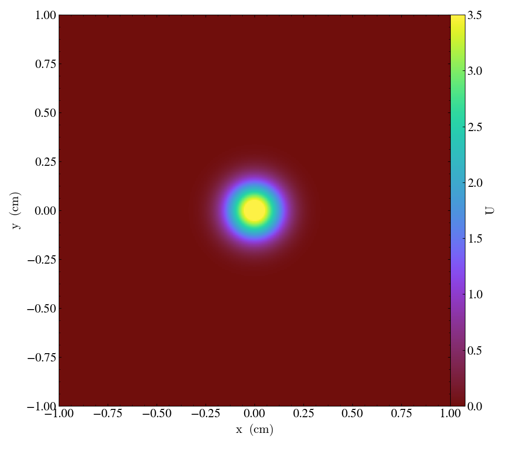 | 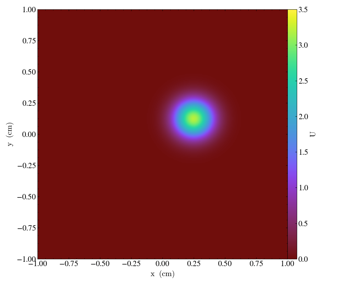 | 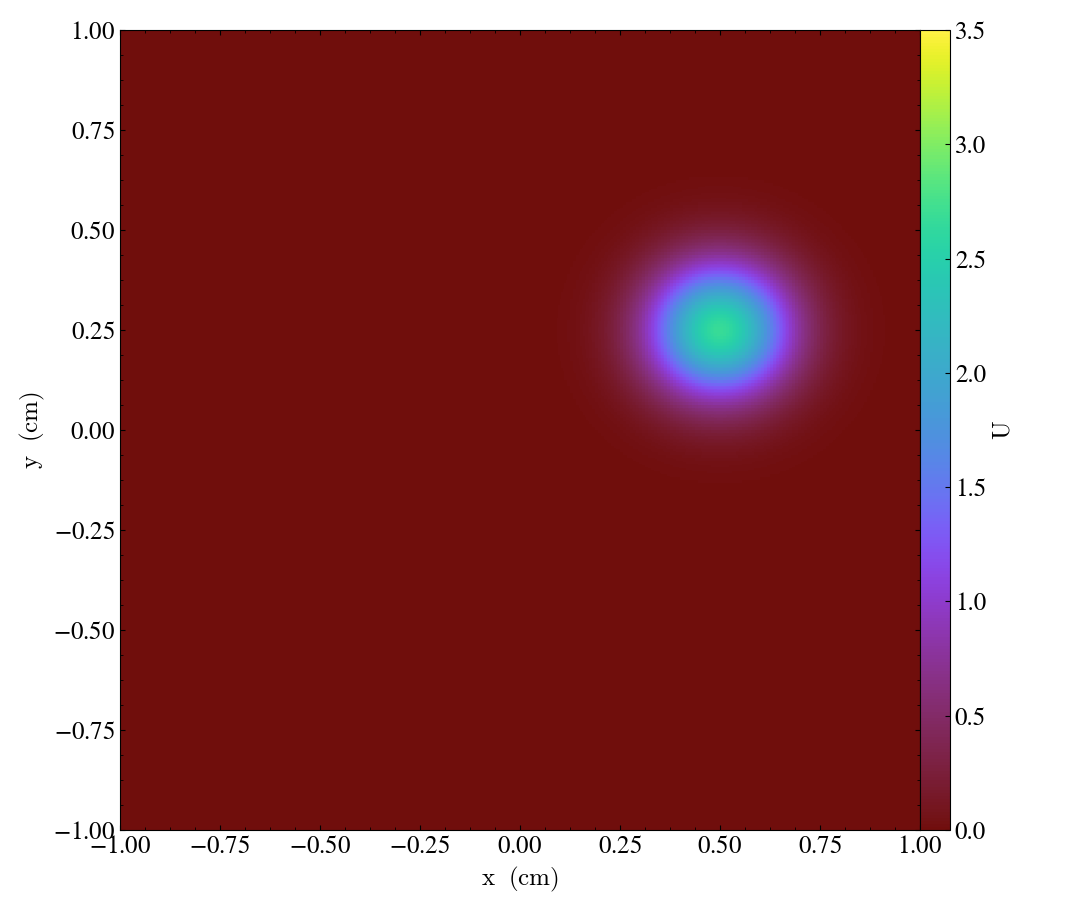 | 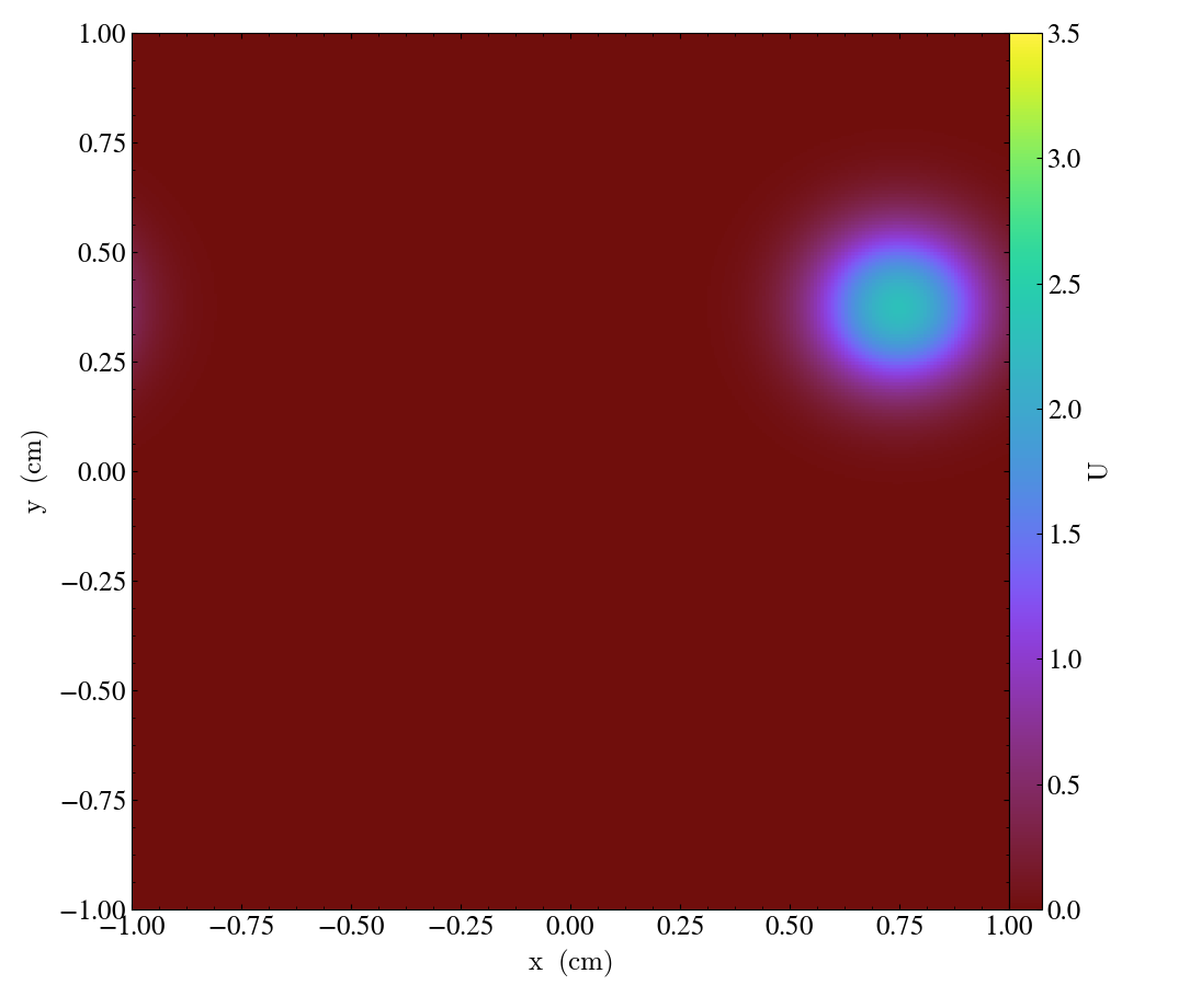 |
We will break apart our investigation of this problem into the following three phases:
- Explicit time integration (
HandsOn1.exe)
(lunch break)
Implicit / IMEX time integration (
HandsOn2.exe)Preconditioning (
HandsOn3.exe)
Getting help
You can get help on all the command-line options to these applications with the help=1 argument for any of these executables, e.g.,
./HandsOn1.exe help=1
MPI initialized with 1 MPI processes
AMReX (19.07) initialized

Usage: HandsOn1.exe [fname] [options]
Options:
  help=1
    Print this help message and exit.
  plot_int=<int>
    enable (1) or disable (0) plots [default=0].
  arkode_order=<int>
    ARKStep method order [default=4].
  fixed_dt=<float>
    use a fixed time step size (if value > 0.0) [default=-1.0].
  rtol=<float>
    relative tolerance for time step adaptivity [default=1e-4].
  atol=<float>
    absolute tolerance for time step adaptivity [default=1e-9].
  tfinal=<float>
    final integration time [default=1e4].
  dtout=<float>
    time between outputs [default=tfinal].
  max_steps=<int>
    maximum number of internal steps between outputs [default=10000].
  write_diag=<int>
    output ARKStep time step adaptivity diagnostics to a file [default=1].
  n_cell=<int>
    number of cells on each side of the square domain [default=128].
  max_grid_size=<int>
    max size of boxes in box array [default=64].
  advCoeffx=<float>
    advection speed in the x-direction [default=5e-4].
  advCoeffy=<float>
    advection speed in the y-direction [default=2.5e-4].
  diffCoeffx=<float>
    diffusion coefficient in the x-direction [default=1e-6].
  diffCoeffy=<float>
    diffusion coefficient in the y-direction [default=1e-6].

If a file name 'fname' is provided, it will be parsed for each of the above
options.  If an option is specified in both the input file and on the
command line, then the command line option takes precedence.
Cleaning up
At any time, you can remove all of the solution output files and ARKode temporal adaptivity diagnostics files with the command
make pltclean
Hands-on lesson 1 – Explicit time integration (HandsOn1.exe)
This lesson will explore the following topics:
a. Problem specification – vector wrapper and right-hand side functions
b. Fixed time-stepping (exploration of linear stability)
c. Adaptive time-stepping
d. Time integrator order of accuracy
Problem specification
There are essentially only three steps required to use SUNDIALS with an existing simulation code:
Create a thin
N_Vectorwrapper for your existing data structures, so that SUNDIALS can think of them as “vectors,” and perform standard algebraic operations directly on your data:clone a vector to create work arrays
linear combination: \(\vec{z} \gets a\vec{x} + b\vec{y}\)
fill with constant: \(z_i \gets c, \; i=0,\ldots,N-1\)
componentwise multiplication: \(\vec{z} \gets \vec{x} .* \vec{y}\)
vector scale: \(\vec{z} \gets c \vec{x}\)
norm and inner-product computations: \(\|\vec{x}\|_\infty\), \(\left<\vec{x},\vec{y}\right>\), etc.
…
An example of this for the native AMReX
MultiFabdata structure may be found in the files shared/NVector_Multifab.h and shared/NVector_Multifab.cpp.Create a function that computes the problem-defining ODE right-hand side function on your
N_Vectordata (or for KINSOL, the problem-defining nonlinear residual function). Here, we implement the advection-diffusion right-hand side function, \[f(t,u) = -\vec{a} \cdot \nabla u + \nabla \cdot ( D \nabla u )\]in
int ComputeRhsAdvDiff(Real t, N_Vector nv_sol, N_Vector nv_rhs, void* data)found in the file shared/Utilities.cpp.
Use SUNDIALS to integrate your ODE/DAE or solve your nonlinear system:
Instantiate and fill an
N_Vectorfor your initial conditions, \(u_0(x,y)\) or your initial guess to the nonlinear solve. In our example this is done here.Create the time integrator memory structure, providing both the initial condition vector \(u_0(x,y)\) and the problem-defining function \(f(t,u)\). In our example, these are done here.
Call the SUNDIALS solver to evolve the problem over a series of time sub-intervals, or to solve the nonlinear problem. Our example does this in a loop here.
Linear stability
Run the first hands-on code using its default parameters (note that this uses a mesh size of \(128^2\) and fixed time step size of 5.0),
./HandsOn1.exe inputs-1
and compare the final result against a stored reference solution (on a \(128^2\) grid),
fcompare.gnu.ex plt00001/ reference_solution/
Notice that the computed solution error is rather small (since the solution has magnitude \(\mathcal{O}(1)\), errors should be less than 0.1).
Now re-run this hands-on code using a larger time step size of 100.0,
./HandsOn1.exe inputs-1 fixed_dt=100.0
see how much faster the code ran! However, now check the accuracy of the computed solution,
fcompare.gnu.ex plt00001/ reference_solution/
and note the reported error of \(10^{98}\).
At this mesh size, the explicit algorithm is unstable for a time step size of 100, but is stable for a time step size of 5.
Run the code a few more times – what is the largest stable time step size that you can find?
Temporal adaptivity
With this executable, we may switch to adaptive time-stepping (with the default tolerances, \(rtol=10^{-4}\) and \(atol=10^{-9}\)) by specifying fixed_dt=0,
./HandsOn1.exe inputs-1 fixed_dt=0
fcompare.gnu.ex plt00001/ reference_solution/
note how rapidly the executable finishes, providing a solution that is both stable and accurate to within the specified tolerances!
Run the accompanying Python script process_ARKStep_diags.py to view some overall time adaptivity statistics and generate plots of the time step size history,
./process_ARKStep_diags.py HandsOn1_diagnostics.txt
display h_vs_iter.png
notice how rapidly the adaptive time-stepper finds the CFL stability limit. Also notice that the adaptivity algorithm periodically attempts to increase the time step size to investigate whether this stability limit has changed; however, the raw percentage of these failed steps remains rather small.
Run the code a few more times with various values of rtol – how well does the adaptivity algorithm produce solutions within the desired tolerances? How do the number of time steps change as different tolerances are requested?
Integrator order and efficiency
ARKode defaults to a fourth-order accurate Runge–Kutta method, but many others are included (explicit methods have available orders 2 through 8). Alternate orders of accuracy may be run with the arkode_order option, e.g.,
./HandsOn1.exe inputs-1 fixed_dt=0 arkode_order=8
fcompare.gnu.ex plt00001/ reference_solution/
note the dramatic decrease in overall time steps (457 vs 258), but the accompanying increase in total RHS evaluations (2865 vs 3773). Although higher-order methods may indeed utilize larger step sizes (both for accuracy and frequently stability), those come at the cost of increased work per step.
Run the code a few more times with various values of arkode_order for a fixed value of rtol – what is the most “efficient” overall method for this problem at this tolerance?
Hands-on lesson 2 – Implicit / IMEX time integration (HandsOn2.exe)
This lesson will explore the following topics:
a. Specification of algebraic solver algorithms (nonlinear and linear)
b. Fixed time-stepping (exploration of linear stability)
c. Adaptive time-stepping
d. Newton vs accelerated fixed-point nonlinear solver
e. Implicit-explicit partitioning
Specification of algebraic solvers
Once your code is set up to run an explicit method, it is not difficult to switch to an implicit or IMEX solver. All of the relevant changes for this in our examples today are in the file HandsOn2.cpp, and are indicated by the comment ***** UPDATED FROM HandsOn1 *****. The main steps are:
Move specification of the ODE right-hand side function to the implicit argument when creating the integrator, or supply separate routines that should be used for the IMEX splitting of the ODE right-hand side.
This is done here in our example, where we either supply
ComputeRhsAdvDiff()for fully implicit integration, or specifies two routinesComputeRhsAdv()andComputeRhsDiff()for an IMEX splitting of the ODE right-hand side.To use the default Newton nonlinear solver, you must specify which linear solver module should be used to solve the inner linear systems of equations.
In our example, we create and attach an un-preconditioned GMRES iterative linear solver for this purpose here.
Alternately, you may select an alternate nonlinear solver module to use instead of Newton.
In our example, if requested we attach an accelerated fixed-point nonlinear solver (with no inner linear solver needed) here.
Linear stability revisited
Run the second hands-on code using its default parameters (note that this also uses a mesh size of \(128^2\) and fixed time step size of 5.0),
./HandsOn2.exe inputs-2
fcompare.gnu.ex plt00001/ reference_solution/
note that this takes significantly longer than HandsOn1.exe with the same time step size
Now re-run using the larger time step size of 100.0,
./HandsOn2.exe inputs-2 fixed_dt=100.0
fcompare.gnu.ex plt00001/ reference_solution/
again this version runs much more quickly, but now the results are usable!
This algorithm is fully-implicit (and in fact, it is A-stable), so linear instability was not a problem.
Run the code a few more times with larger time step sizes, checking the overall solution error each time – can you find an unstable step size? Are there step sizes where the code may be stable, but are so large that the nonlinear and/or linear solver fails to converge?
Temporal adaptivity revisited
As with the previous hands-on exercise, we may switch to adaptive time-stepping (with the default tolerances, \(rtol=10^{-4}\) and \(atol=10^{-9}\)) by specifying fixed_dt=0,
./HandsOn2.exe inputs-2 fixed_dt=0
Compute the solution error, and determine the adaptive time-stepping statistics as before,
fcompare.gnu.ex plt00001/ reference_solution/
./process_ARKStep_diags.py HandsOn2_diagnostics.txt
display h_vs_iter.png
How does that average step size for this tolerance compare against the average step size of HandsOn1.exe for the same tolerances?
The solution becomes smoother and decays toward zero as time goes on, making the initial guesses for each Newton and GMRES iteration more accurate, and the systems easier to solve, so ARKode gradually increases the step size as it is able.
Run the code a few more times with various values of rtol – how well does the adaptivity algorithm produce solutions within the desired tolerances? How do the number of time steps change as different tolerances are requested? Is this algorithm more useful than the fully explicit approach when loose tolerances (e.g., rtol=1e-1) are requested?
Nonlinear solvers
As mentioned above, HandsOn2.exe defaults to solving implicit stages using an inexact Newton nonlinear solver. We may switch this nonlinear solver algorithm to an accelerated fixed-point nonlinear solver (with the default acceleration subspace size, nls_fp_iter=3) by specifying nls_method=1; since fixed-point methods typically converge more slowly than Newton-based methods, we will also increase the allowed number of nonlinear iterations by specifying nls_max_iter=20,
./HandsOn2.exe inputs-2 fixed_dt=0 nls_method=1 nls_max_iter=20
fcompare.gnu.ex plt00001/ reference_solution/
How do the total number of implicit RHS function calls, solution accuracy, number of time steps, and total runtime compare against an identical run using the inexact Newton nonlinear solver?
Since the inexact Newton and accelerated fixed-point solvers use different internal algorithms (linear algebra, vs “acceleration”), the per-iteration costs of these methods vary substantially.
Run the code a few more times with various values of nls_fp_acc (e.g., 0 through 6) to determine whether there is a more ‘optimal’ value of the acceleration subspace size for this problem.
IMEX partitioning
By default, HandsOn2.exe uses a fully implicit formulation of the problem. However, this can instead be run with the advection terms \(\vec{a} \cdot \nabla u\) treated explicitly by specifying rhs_adv=2,
./HandsOn2.exe inputs-2 rhs_adv=2
fcompare.gnu.ex plt00001/ reference_solution/
For comparison, re-run an identical test but with fully-implicit treatment,
./HandsOn2.exe inputs-2
fcompare.gnu.ex plt00001/ reference_solution/
Do you notice any efficiency or accuracy differences between fully implicit and IMEX formulations with these fixed time-step tests?
Since the explicit portion need only be computed once per stage, but the implicit portion must be repeatedly called at each stage during the nonlinear solver algorithm, we should expect ARK-IMEX methods to always evalute Fi more often than Fe.
Now that we again have an explicit portion of the problem, we should expect the time step size to be CFL-limited. Run the IMEX version a few times with various fixed time step sizes (the fixed_dt argument), checking the overall solution error each time – can you find an unstable step size?
Since diffusion is now treated implicitly, the CFL-limited step size is now determined only by the advection terms. As these are qualitatively different than the diffusion terms, we should expect different stability limitations.
Hands-on lesson 3 – Preconditioning (HandsOn3.exe)
This lesson will explore the following topics:
a. Preconditioner specification
b. Performance for IMEX time integrators
c. Performance for fully implicit time integrators
The file HandsOn3.cpp is nearly identical to the previous versions (with relevant changes indicated by the comment ***** UPDATED FROM HandsOn2 *****). We note, however, that it’s default parameters differ slightly from the previous versions:
it defaults to adaptive time-stepping (with the same default tolerances)
it defaults to IMEX mode, with advection treated explicitly
it defaults to using the preconditioner (discussed below).
Preconditioner specification
Perhaps the most challenging (and most critical) component for a scalable implicit or IMEX time integrator is the creation of an effective, efficient, and scalable preconditioner to accelerate the iterative linear solvers (more on this by the next speakers). This requires three steps:
Create preconditioner “setup” and “solve” routines that prepare any data structures necessary to perform preconditioning (called infrequently) and apply the preconditioner (called frequently), respectively.
Here, we create the routines precondition_setup and preconditioner_solve, that employ a scalable geometric multigrid solver for only the diffusion portion of the problem, \(\nabla \cdot ( D \nabla u )\). This should be a perfect preconditioner when running in IMEX mode, but will only be approximate when running a fully implicit formulation of the problem.
Supply the preconditioning routines to the integrator.
In our example, when creating the GMRES linear solver, we notify it to use left preconditioning here. We then attach the
precondition_setupandprecondition_solveroutines to the integrator here.
Performance with IMEX integration
Run HandsOn3.exe using the default parameters,
./HandsOn3.exe inputs-3
and again with preconditioning disabled,
./HandsOn3.exe inputs-3 use_preconditioner=0
note that the preconditioned version takes longer to run on this coarse problem, but shows significant improvements in the overall number of linear solver iterations.
We only ran this code on a very coarse problem, where the un-preconditioned GMRES solver proved “sufficient” for solving the Newton linear systems; however at larger scales the linear system becomes “ill-conditioned,” requiring a preconditioner for convergence. Related – the preconditioned solver should be algorithmically scalable, so at some point we should expect the preconditioned version to out-perform the unpreconditioned version.
Performance with fully implicit integration
Re-run HandsOn3.exe using a fully-implicit problem formulation,
./HandsOn3.exe inputs-3 rhs_adv=1
Recall that this preconditioner only ‘preconditions’ the diffusion portion of the problem, so when run in a fully-implicit manner the implicit advection terms are left un-preconditioned. Is this discrepancy noticeable when comparing the solver statistics (number of time steps, total linear iterations, etc.)?
In the evening hands-on session (below), you can explore the scalability and efficiency of both the un-preconditioned and preconditioned versions of this hands-on lesson.
Out-brief
We have used AMReX and SUNDIALS as a demonstration vehicle for illustrating the value of robust time integration methods in numerical algorithms. In particular, we have used the ARKode’s ARKStep time integration module from SUNDIALS to explore a range of questions related to time integration and nonlinear solvers:
the benefits of adaptive (vs fixed) time stepping for both performance and robustness of a simulation code,
the effects of the order of the time integration method on method efficiency,
the tradeoffs between more powerful (but costly) Newton-based nonlinear solvers and cheaper but more slowly-convergent fixed-point nonlinear solvers,
the increased cost but increased scalability offered through use of advanced preconditioning methods, and
the choice of IMEX partitioning in time discretization.
We note that our use of adaptivity here was confined to the time discretization only. Other lessons here demonstrate the advantages of spatial adaptation as well (e.g., AMR).
We further note that we have barely scratched the surface of linear solver algorithms; while GMRES with geometric multigrid preconditioning remains a top choice of many large-scale applications, other lessons here will focus on alternatives that can work for much broader classes of problems.
Finally, we note that the application demonstrated here can be run on much larger spatial meshes and parallel architectures than those tested here.
Evening hands-on session
Each of the following tasks are independent of one another. Choose one to explore in detail during this evening session (or if interested, you may do multiple).
(10 points) Examine the explicit stability boundary for
HandsOn1.exeas the mesh sizen_cellis changed to 256 and 512. Do the same forHandsOn2.exewhen running in IMEX mode (with explicit advection). Determine whether the stability boundaries for these problems are \(\Delta t_n \propto \Delta x\) or \(\Delta t_n \propto \Delta x^2\).(5 points) Explore the weak scalability of
HandsOn3.exeboth with and without preconditioning. Here, use from 1 to 36 MPI tasks, with a base grid of \(128^2\) per MPI task, and retain the default temporal adaptivity. The choice of IMEX vs fully implicit is yours. It is recommended that you use the batch queue instead of running interactively. Produce a weak scaling plot with these results.(10 points) Add a simple ‘reaction’ term to the problem, e.g. \[\frac{\partial u}{\partial t} + \vec{a} \cdot \nabla u - \nabla \cdot ( D \nabla u ) = -u^2\]
You may add this to either the explicit or implicit portions of the right-hand side; how well does the existing preconditioner do after this is added?
When you are done, be sure to submit a Show Your Work using the hands-on activity name Time Integrators and upload evidence of your completed solutions.