Meshing and Discretization with AMReX
![]()
At a Glance
| Questions | Objectives | Key Points |
| How does Adaptive Mesh Refinement (AMR) work and when would I want it? | Understand AMR applicability, benefits and trade-offs. | AMR is a flexible approach for achieving science goals. |
| How does AMReX do AMR? | Understand AMReX provides functionality as a software framework. | Simulations are coded with AMReX data structures and functions; your science is still your code. |
| Would AMReX be useful for my application? | Understand conceptual requirements and benefits of running with AMReX. | AMReX provides support for AMR, Embedded Boundaries, Particles and more on a variety of heterogeneous architectures. |
Setup Instructions For AMReX Tutorials
- Log into the Theta login node with your username (replace “elvis”):
ssh -A elvis@theta.alcf.anl.gov - In your home folder, create a local copy of the track 5 numerical examples:
cd ~ rsync -a /grand/ATPESC2022/EXAMPLES/track-5-numerical . - To access ThetaGPU resources, transfer to a GPU service node:
ssh thetagpusn1 # or thetagpusn2 - From the GPU service node, request a single-gpu reservation:
qsub -I -q single-gpu -t 60 -n 1 -A ATPESC2022 - Load OpenMPI:
module load openmpi/openmpi-4.1.4_ucx-1.12.1_gcc-9.4.0 - Change to the AMReX examples directory:
cd track-5-numerical/EXAMPLES/amrex - Setup several environment variables and path by
sourcing the
amrex_setup_env.shscript:source amrex_setup_env.sh
Science Goal
To motivate our discussion of adaptive mesh refinement we will consider the flow of a dye in water around a cylinder. See the video below:
|
|---|
| https://www.youtube.com/watch?v=KiBrKzykwO8 |
We want to develop a fluid simulation that captures the behavior seen in this experiment. To capture the interactions carefully, we plan on doing a large and detailed simulation and will therefore be limited by computational resources and time to solution. Moreover, we know that our focus is on the water-dye boundary, and not on the water as a whole, so an approach with adaptive mesh refinement would provide benefits. As a first step in developing this simulation, we consider a simplified problem, the flow of the dye without a cylinder.
AMR101: Multi-Level Scalar Advection
FEATURES:
- Mesh Data
- Dynamic Adaptive Mesh Refinement
- Scalable Parallel Computation
Mathematical Formulation
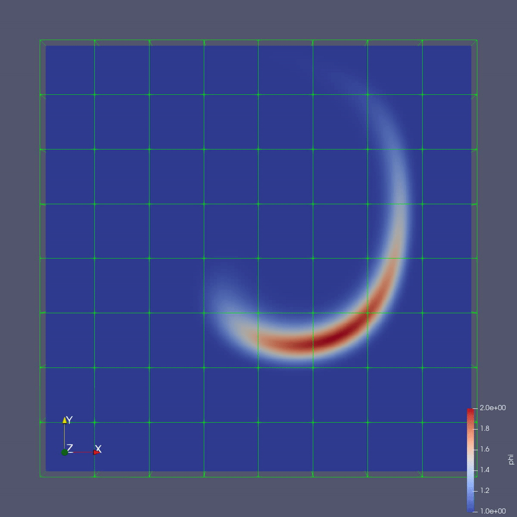
Let \(\phi\) represent the concentration of dye in the water in in a thin incompressible fluid that is spinning clock-wise and then counter-clockwise with a prescribed motion (This is useful for verifying our algorithms). We consider the dye to be a passive tracer that is advected by the fluid velocity and the fluid thin enough that we can model this as two-dimensional motion.
In other words, we want to solve for \(\phi(x,y,t)\) by evolving \[\frac{\partial \phi}{\partial t} + \nabla \cdot (\bf{u^{spec}} \phi) = 0\]
in time (\(t\)), where the velocity \({\bf{u^{spec}}} = (u,v)\) is a divergence-free field computed by defining \[\psi(i,j) = \sin^2(\pi x) \sin^2(\pi y) \cos (\pi t / 2) / \pi\]
and defining \[u = -\frac{\partial \psi}{\partial y}, v = \frac{\partial \psi}{\partial x}.\]
Note that because \({\bf{u^{spec}}}\) is defined as the curl of a scalar field, it is analytically divergence-free
In this example we’ll be using AMR to resolve the scalar field since the location of the dye is what we care most about.
Algorithm
To update the solution in a patch at a given level, we compute fluxes (\({\bf u^{spec}} \phi\)) on each face, and difference the fluxes to create the update to phi. The update routine in the code looks like
  // Do a conservative update
  {
    phi_out(i,j,k) = phi_in(i,j,k) +
                ( AMREX_D_TERM( (flxx(i,j,k) - flxx(i+1,j,k)) * dtdx[0],
                              + (flxy(i,j,k) - flxy(i,j+1,k)) * dtdx[1],
                              + (flxz(i,j,k) - flxz(i,j,k+1)) * dtdx[2] ) );
  }
In this routine we use the macro AMREX_D_TERM so that we can write dimension-independent code;
in 3D this returns the flux differences in all three directions, but in 2D it does not include
the z-fluxes.
Adaptive Mesh Refinement
Adaptive mesh refinement focuses computation on the areas of interest. In this example, our interest is in the water-dye boundary and not water in other places in the domain. Adaptive mesh refinement will allow us to set grids in this area with smaller dimensions and/or small time steps. The result is areas with finer grids have results with higher accuracy.
Developing a code that is capable of adaptive mesh refinement, broadly speaking, requires:
- Knowing how to advance the solution one patch at a time.
- Knowing the matching conditions at coarse/fine interfaces. Below we show a snippet of code in this simulation written with the AMReX framework for generating a finer grid level from a coarser one.
// Make a new level using provided BoxArray and DistributionMapping and
// fill with interpolated coarse level data.
// overrides the pure virtual function in AmrCore
void
AmrCoreAdv::MakeNewLevelFromCoarse (int lev, Real time, const BoxArray& ba,
                    const DistributionMapping& dm)
{
    const int ncomp = phi_new[lev-1].nComp();
    const int nghost = phi_new[lev-1].nGrow();

    phi_new[lev].define(ba, dm, ncomp, nghost);
    phi_old[lev].define(ba, dm, ncomp, nghost);

    t_new[lev] = time;
    t_old[lev] = time - 1.e200;

    // This clears the old MultiFab and allocates the new one
    for (int idim = 0; idim < AMREX_SPACEDIM; idim++)
    {
    facevel[lev][idim] = MultiFab(amrex::convert(ba,IntVect::TheDimensionVector(idim)), dm, 1, 1);
    }

    if (lev > 0 && do_reflux) {
    flux_reg[lev].reset(new FluxRegister(ba, dm, refRatio(lev-1), lev, ncomp));
    }

    FillCoarsePatch(lev, time, phi_new[lev], 0, ncomp);
}
Running the Code
To run the code navigate to the directory with your copy of the AMReX examples.
cd track-5-numerical/amrex/AMReX_Amr101/Exec
In this directory you’ll see:
main3d.gnu.MPI.ex -- the 3D executable -- this has been built with MPI

inputs -- a file specifying simulatin parameters
To run in serial:
./main3d.gnu.MPI.ex inputs
To run in parallel, for example on 4 ranks:
mpiexec -n 4 ./main3d.gnu.MPI.ex inputs
Inputs File
The following parameters can be set at run-time – these are currently set in the inputs file but you can also set them on the command line.
stop_time          = 2.0                # the final time (if we have not exceeded number of steps)
max_step           = 100000              # the maximum number of steps (if we have not exceeded stop_time)

amr.n_cell         = 64 64 8             # number of cells at the coarsest AMR level in each coordinate direction

amr.max_grid_size  = 16                  # the maximum number of cells in any direction in a single grid

amr.plot_int       = 10                  # frequency of writing plotfiles

adv.cfl            = 0.9                 # cfl number to be used for computing the time step

adv.phierr = 1.01  1.1  1.5              # regridding criteria  at each level
This inputs file specifies a base grid of 64 x 64 x 8 cells, made up of 16 subgrids each with 16x16x8 cells.
Here is also where we tell the code to refine based on the magnitude of \(\phi\). We set the
threshold level by level. If \(\phi > 1.01\) then we want to refine at least once; if \(\phi > 1.1\) we
want to resolve \(\phi\) with two levels of refinement, and if \(\phi > 1.5\) we want even more refinement.
Boundaries are set to be periodic in all directions (Not shown above).
Simulation Output
Note that you can see the total runtime by looking at the line at the end of your run that says,
Total Time:
and you can check conservation of \(\phi\) by checking the line that prints, e.g.
Coarse STEP 8 ends. TIME = 0.007031485953 DT = 0.0008789650903 Sum(Phi) = 540755.0014
“Sum(Phi)” is the sum of \(\phi\) over all the cells at the coarsest level.
Visualizing the Results
For convenience we created a python script powered by ParaView 5.9 to render the AMReX plotfiles. FFmpeg is then used to stitch the images into a movie and gif. To generate a movie from the plotfiles type:
pvbatch movie_amr101.py
This will generate two files, amr101_3D.avi and amr101_3D.gif.
To view the files you can copy them to your local machine and view
them with scp. Open a terminal on your local machine and move the folder where you want
to download the mp4 and gif. Then type:
scp elvis@theta.alcf.anl.gov:~/track-5-numerical/AMReX_Amr101/amr101_3D* .
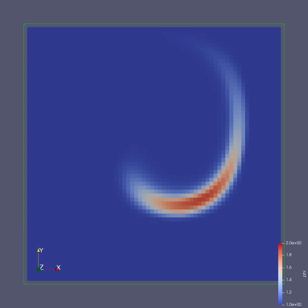
The image below shows a slice through a 3D run with 64x64x8 cells at the coarsest level and three finer levels (4 total levels).
To plot the files manually with a local copy of ParaView see the details below:
To do the same thing with ParaView 5.9 manually (if, e.g. you have the plotfiles
on your local machine and want to experiment):
You are now ready to play the movie! See the "VCR-like" controls at the top. Click the play button.
Activity
Try the following:
-
Run
AMReX_Amr101with and without adaptive mesh refinement and consider how the differing runs compare. -
Run
AMReX_Amr101in parallel with different numbers of MPI Ranks and compare results. Also try using theinputsinput file andinputs_for_scalinginput file.
Key Observations:
-
Adaptive mesh refinement can focus computational resources for higher resolution and lower runtimes.
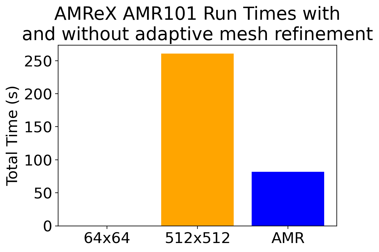
Comparison of three different runs. The first two show the result without adaptive mesh refinement. Here, the lowest resolution run with 64x64x8 is the fastest but captures the least detail. The second run has a resolution of 512x512x8 but it takes almost three times longer than the last run. The last run with adaptive mesh refinement enabled, has 4 levels, with a resolutions that vary from 64x64x8 to 512x512x64. The animations follow the same order as the bar plot above. From left to right, 64x64x8, and 512x512x8 without refinement, and a run with adaptive mesh refinement.

-
Efficient MPI scaling reduces runtimes but requires thought.
AMR101 Runtimes on Theta MPI Ranks Total Time 1 23.940 2 12.964 4 6.844 8 3.764 16 2.174 32 1.217 64 0.849 128 0.621
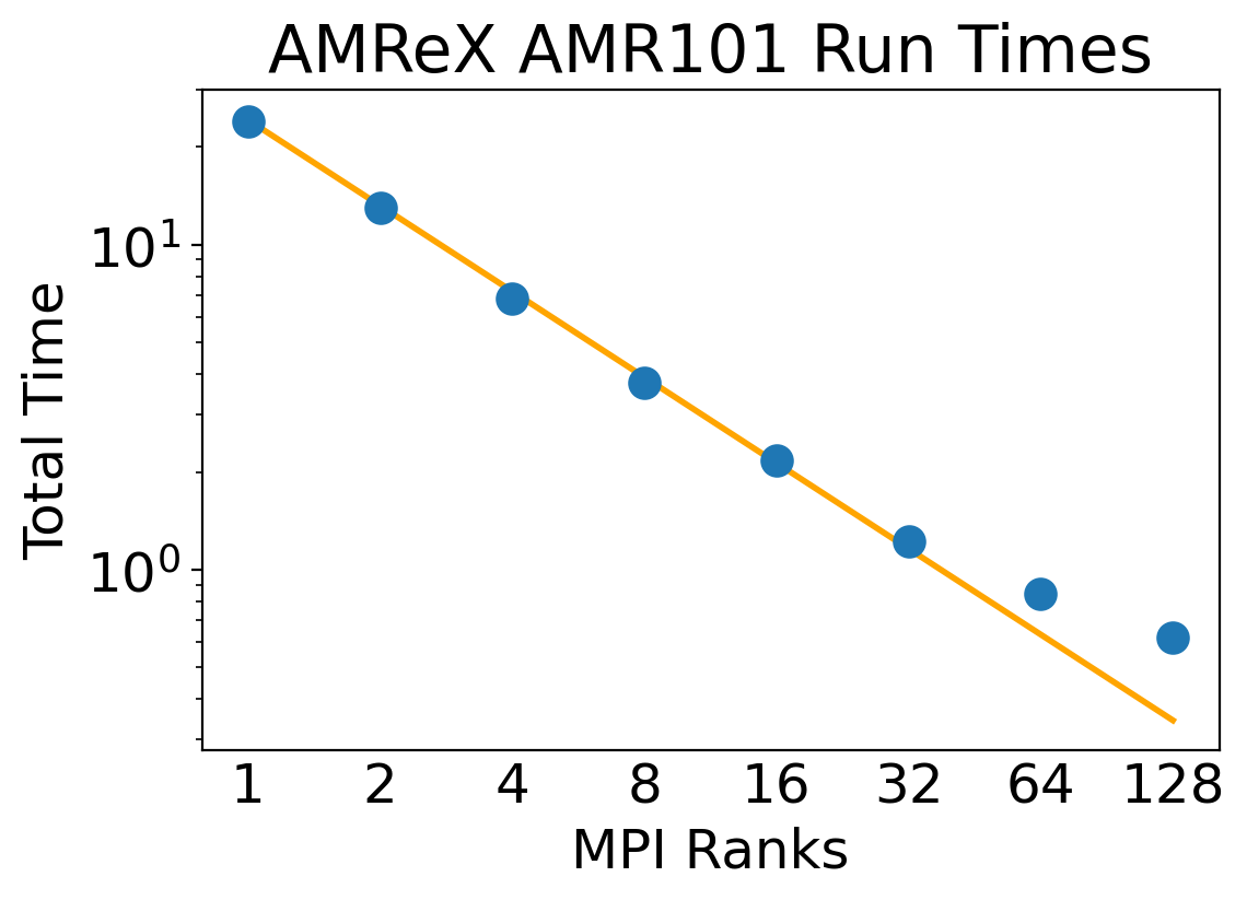 The figure above shows the result of running,
    mpiexec -n 1 ./main3d.gnu.MPI.ex inputs_for_scaling
    mpiexec -n 2 ./main3d.gnu.MPI.ex inputs_for_scaling
    mpiexec -n 4 ./main3d.gnu.MPI.ex inputs_for_scaling
  ...
with different numbers of MPI ranks.
Run times quickly decrease with the number of MPI Ranks, demonstrating
good scaling. However, as the number of ranks gets above 64,
the amount of decrease slows down.
This can be due to a number of reasons, such as communication cost, or
not enough work for each rank. In this case, its likely the former.
Parallelism with GPUs
Suppose at this point in your project, you find that you have written a successful CPU code and then you discover you will have access to a GPU enabled machine. Typically, it may be difficult to adapt your code to take advantage of these resources. And while there are compatibility layers out there, the AMReX framework is already poised to take advantage of GPUs with very little change to the code. To illustrate this point, the same AMReX source code from our CPU-code can be recompiled to use a GPU backend where appropriate.
The example section of the AMReX_Amr101 source code below shows C++ code that can be optimized for MPI, OpenMP, and GPU computations at compile time.
#ifdef _OPENMP
#pragma omp parallel if(Gpu::notInLaunchRegion())
#endif
    {

        for (MFIter mfi(state,TilingIfNotGPU()); mfi.isValid(); ++mfi)
        {
            const Box& bx  = mfi.tilebox();
            const auto statefab = state.array(mfi);
            const auto tagfab  = tags.array(mfi);
            Real phierror = phierr[lev];

            amrex::ParallelFor(bx,
            [=] AMREX_GPU_DEVICE (int i, int j, int k) noexcept
            {
                state_error(i, j, k, tagfab, statefab, phierror, tagval);
            });
        }
    }
This AMReX construction adapts to several forms of parallelism. When MPI is used, it will distribute the work among MPI ranks. When OpenMP is enabled, work is distributed among threads. When a GPU backend is enabled, this computation will be done on the GPU. AMReX functionality is flexible enough that this can be adapted for NVidia, AMD, or Intel GPUs without code changes.
For convenience, there is a binary pre-compiled with CUDA support in the AMReX_Amr101/Exec
folder, ./main3d.gnu.CUDA.MPI.ex. If one wanted to compile the source code with CUDA,
the command would be:
make DIM=3 USE_MPI=TRUE USE_CUDA=TRUE CUDA_ARCH=80
Activity
- Try running the GPU enabled version and compare runtimes.
Key Observations
-
Running on GPUs did not require changes to the code.
-
Running on GPUs was fast.
AMR102: Advection of Particles Around Obstacles
FEATURES:
- Mesh data with Embedded Boundaries
- Linear Solvers (Multigrid)
- Particle-Mesh Interpolation
Next we will add complexity with particles and embedded boundaries (EB).
Mathematical Problem Formulation
Recall our previous problem of the drop of dye in a thin incompressible fluid that is spinning clock-wise then counter-clockwise with a prescribed motion.
Now instead of advecting the dye as a scalar quantity defined on the mesh (the continuum representation), we define the dye as a collection of particles that are advected by the fluid velocity.
Again we consider the fluid thin enough that we can model this as two-dimensional motion.
To make things even more interesting, there is now an object in the flow, in this case a cylinder. It would be very difficult to analytically specify the flow field around the object, so instead we project the velocity field so that the resulting field represents incompressible flow around the object.
Projecting the Velocity for Incompressible Flow around the Cylinder
Mathematically, projecting the specified velocity field means solving \[\nabla \cdot (\beta \nabla \xi) = \nabla \cdot \bf{u^{spec}}\]
and setting \[\bf{u} = \bf{u^{spec}} - \beta \nabla \xi\]
To solve this variable coefficient Poisson equation, we use the native AMReX geometric multigrid solver. In our case \(\beta = 1 / \rho = 1\) since we are assuming constant density \(\rho.\)
Note that for this example we are solving everything at a single level for convenience, but linear solvers, EB and particles all have full multi-level functionality.
In each timestep we compute the projected velocity field, advect the particles with this velocity, then interpolate the particles onto the mesh to determine \(\phi(x,y,z)\).
Particle-In-Cell Algorithm for Advecting \(\phi\)
We achieve conservation by interpreting the scalar \(\phi\) as the number density of physical dye particles in the fluid, and we represent these physical particles by “computational” particles \(p\). Each particle \(p\) stores a weight \(w_p\) equal to the number of physical dye particles it represents.
This allows us to define particle-mesh interpolation that converts \(\phi(x,y,z)\) to a set of particles with weights \(w_p\). First, we interpolate \(\phi(x,y,z)\) to \(\phi_p\) at each particle location by calculating: \[\phi_p = \sum_i \sum_j \sum_k S_x \cdot S_y \cdot S_z \cdot \phi(i,j,k)\]
where in the above, \(S_{x,y,z}\) are called shape factors, determined by the particle-in-cell interpolation scheme we wish to use.
The simplest interpolation is nearest grid point (NGP), where \(S_{x,y,z} = 1\) if the particle \(p\) is within cell \((i,j,k)\) and \(S_{x,y,z} = 0\) otherwise. An alternative is linear interpolation called cloud-in-cell (CIC), where the shape factors are determined by volume-weighting the particle’s contribution to/from the nearest 8 cells (in 3D).
Once we have interpolated \(\phi(x,y,z)\) to the particle to get \(\phi_p\), we scale it by the volume per particle to get the number of physical dye particles that our computational particle represents. Here, \(n_{ppc}\) is the number of computational particles per cell. \[w_p = \phi_p \cdot \dfrac{dx dy dz}{n_{ppc}}\]
To go back from the particle representation to the grid representation, we reverse this procedure by summing up the number of physical dye particles in each grid cell and dividing by the grid cell volume. This recovers the number density \(\phi(x,y,z)\). \[\phi(i,j,k) = \dfrac{1}{dx dy dz} \cdot \sum_p S_x \cdot S_y \cdot S_z \cdot w_p\]
This approach is the basis for Particle-In-Cell (PIC) methods in a variety of fields, and in this tutorial you can experiment with the number of particles per cell and interpolation scheme to see how well you can resolve the dye advection.
Running the code
To run the code navigate to the directory with your copy of the AMReX examples.
cd track-5-numerical/amrex/AMReX_Amr102/Exec
In this directory you’ll see
main3d.gnu.MPI.ex -- the 3D executable -- this has been built with MPI

inputs -- an inputs file
As before, to run the 3D code in serial:
./main3d.gnu.MPI.ex inputs
To run in parallel, for example on 4 ranks:
mpiexec -n 4 ./main3d.gnu.MPI.ex inputs
Similar to the last example, the following parameters can be set at run-time – these are currently set in the inputs file.
stop_time =  2.0                         # the final time (if we have not exceeded number of steps)
max_step  = 200                          # the maximum number of steps (if we have not exceeded stop_time)

n_cell = 64                              # number of cells in x- and y-directions; z-dir has 1/8 n_cell (if 3D)

max_grid_size = 32                       # the maximum number of cells in any direction in a single grid

plot_int = 10                            # frequency of writing plotfiles
The size, orientation and location of the cylinder are specified in the inputs file as well:
cylinder.direction = 2                  # cylinder axis aligns with z-axis
cylinder.radius    = 0.1                # cylinder radius
cylinder.center    = 0.7 0.5 0.5        # location of cylinder center (in domain that is unit box in xy plane)

cylinder.internal_flow = false          # we are computing flow around the cylinder, not inside it
Here you can play around with changing the size and location of the cylinder.
The number of particles per cell and particle-mesh interpolation type are also specified in the inputs file:
n_ppc = 100                              # number of particles per cell for representing the fluid

pic_interpolation = 1                    # Particle In Cell interpolation scheme:
                                         # 0 = Nearest Grid Point
                                         # 1 = Cloud In Cell
You can vary the number of particles per cell and interpolation to see how they influence the smoothness of the phi field.
Activity:
Try the following:
- First run
AMReX_Amr102with the defaults. Then look through the inputs file and try changing some of the parameters. How do the runs compare?
Key Observations:
-
How does the solution in the absence of the cylinder compare to our previous solution (where phi was advected as a mesh variable)?
-
Note that at the very end we print the time spent creating the geometrical information. How does this compare to the total run time?
-
Note that for the purposes of visualization, we deposited the particle weights onto the grid. Was phi conserved using this approach?
Visualizing the Results
As in the previous example, we created a python script to render the AMReX plotfiles into a movie and gif. To generate a movie from the plotfiles type:
pvbatch movie_amr102.py
This will generate two files, amr102_3D.mp4 and amr102_3D.gif.
To view the files you can copy them to your local machine and view
them with scp. Open a terminal on your local machine and move the folder where you want
to download the mp4 and gif. Then type:
scp elvis@theta.alcf.anl.gov:~/track-5-numerical/AMReX_Amr101/amr101_3D* .
Notes:
-
To delete old plotfiles before a new run, do
rm -rf plt* -
You can do
realpath amr102_3D.gifto get the movie’s path on ThetaGPU and then copy it to your local machine by doingscp [username]@theta.alcf.anl.gov:[path-to-gif] .
If you’re interested in generating the movies manually, see the details below.
To do the same thing with ParaView 5.8 manually (if, e.g. you have the plotfiles
on your local machine and want to experiment):
There are three types of data from the simulation that we want to load:
To load the mesh data, follow steps 1-10 for plotting phi in the AMR 101 tutorial,
then continue as below to add the EB representation of the cylinder and the particle data.
Instructions to visualize the EB representation of the cylinder:
You should see 1 cylinder with its axis in the z-direction.
Now to load the particles:
You are now ready to play the movie! See the "VCR-like" controls at the top. Click the play button.
Example: AMReX-Pachinko
What Features Are We Using
- EB for obstacles
- Particle-obstacle and particle-wall collisions
The Problem
Have you ever played pachinko?
A pachinko machine is like a vertical pinball machine.
Balls are released at the top of the “playing field”, and bounce off obstacles as they fall.
The object of the game is to “capture” as many balls as possible.
In the AMReX-Pachinko game you can release as many particles as you like at the top of the domain, and the balls will freeze when they hit the bottom so you can see where they landed.
Your goal here is to see if you can cover the floor of the pachinko machine.
(Note that this is not completely realistic – the balls here don’t feel each other so they can overlap.)
Running the Code
The code is located in your copy of the AMReX examples at:
cd track-5-numerical/amrex/AMReX_EB_Pachinko
In this directory you’ll see
main3d.gnu.MPI.ex    -- the executable -- this has been built with MPI

inputs_3d            -- domain size, size of grids, how many time steps, which obstacles...

initial_particles_3d -- initial particle locations  (this name is given in the inputs_3d file)
In this example there is no fluid (or other variable) stored on the mesh but we still sort the particles according to our spatial decomposition of the domain. If we run in parallel with 4 processors, we see the domain decomposition below – this results from using a z-order space-filling curve with the number of cells per grid as the cost function.
For now we freeze the obstacles (although if you look in the code it’s not hard to figure out how to change them!) but we can change the initial particle locations at run-time by editing the initial_particles_3d file.
To run in serial,
./main3d.gnu.MPI.ex inputs_3d
To run in parallel, for example on 4 ranks:
mpiexec -n 4 ./main3d.gnu.MPI.ex inputs_3d
The following parameters can be set at run-time – these are currently set in the inputs_3d file. In this specific example we use only 4 cells in the z-direction regardless of n_cell.
n_cell = 125                          # number of cells in x-direction; we double this in the y-direction
max_grid_size = 25                    # the maximum number of cells in any direction in a single grid

plot_int = 10                         # frequency of writing plotfiles

particle_file = initial_particles_3d  # name of file where we specify the input positions of the particles

time_step = 0.001                     # we take a fixed time step of this size

max_time  = 3.0                       # the final time (if max_time < max_steps * time_step)
max_steps = 100000                    # the maximum number of steps (if max_steps * time_step < max_time))
You can also set values on the command line; for example,
mpiexec -n 4 ./main3d.gnu.MPI.ex inputs_3d particle_file=my_file
will read the particles from a file called “my_file”
The output from your run should look something like this:
********************************************************************
 Let's advect the particles ...
   We'll print a dot every 10 time steps.
********************************************************************

.............................................................................................................................................................................................................................................................................................................

********************************************************************
We've finished moving the particles to time 3
That took 1.145916707 seconds.
********************************************************************
Visualizing the Results
As in the previous example, we created a python script to render the AMReX plotfiles into a movie and gif. To generate a movie from the plotfiles type:
pvbatch movie_pachinko.py
This will generate two files, pachinko.avi and pachinko.gif.
To view the files you can copy them to your local machine and view
them with scp. Open a terminal on your local machine and move the folder where you want
to download the mp4 and gif. Then type:
scp elvis@theta.alcf.anl.gov:~/track-5-numerical/AMReX_Amr101/pachinko* .
If you’re interested in generating the movies manually, see the details below.
There are three types of data from the simulation that we want to load:
Because the EB data and mesh data don't change, we load these separately from the particles.
Instructions to visualize the EB representation of the cylinders:
You should see cylinders with their axes in the z-direction.
Now to add the mesh field:
Now to load the particles:
You are now ready to play the movie! See the "VCR-like" controls at the top. Click the play button.
For fun: if you want to color the particles, make sure "Glyph1" is highlighted, then
change the drop-down menu option (above the calculator row) from "vtkBlockColors" to "cpu" --
if you have run with 4 processes then you will see the particles displayed with different colors.
Further Reading
Download AMReX from GitHub here.
AMReX documentation/tutorials can be found here
Read a Journal of Open Source Software (JOSS) paper on AMReX here