Meshing and Discretization with AMReX
At a Glance
| Questions | Objectives | Key Points |
| What can I do with AMReX? | Understand that “AMR” means more than just “traditional AMR” | AMR + EB + Particles |
| How do I get started? | Understand easy set-up | It’s not hard to get started |
| What time-stepping do I use? | Understand the difference between subcycling and not | It’s a choice |
| How do I visualize AMR results? | Use Visit and Paraview for AMReX vis | Visualization tools exist for AMR data. |
Setup Instructions For AMReX Tutorials
Vis can be finicky on Cooley because there are certain details that we need to set up first:
- Access Cooley with
ssh -X - Vis needs to be run inside an interactive session on a compute node
Recall, to get an interactive session, do, e.g.:
qsub -I -n 1 -t 300 -A ATPESC2021 -q training
- Then in the interactive session, edit your
~/.soft.cooleyfile to contain only the following and then use theresoftcommand:
+mvapich2
+anaconda3-4.0.0
+ffmpeg
@default
- Also in the interactive session, configure the vis tools using the following command:
source /grand/projects/ATPESC2021/EXAMPLES/track-5-numerical/amrex/source_this_file.sh
- When finished with these AMReX tutorials, revise your
~/.soft.cooleyfollowing step 3 here and then doresoftto revert these package changes for other tutorials.
Example: AMR101: Multi-Level Scalar Advection
What Features Are We Using
- Mesh data
- Dynamic AMR with and without subcycling
The Problem
Consider a drop of dye (we’ll define \(\phi\) to be the concentration of dye) in a thin incompressible fluid that is spinning clock-wise then counter-clockwise with a prescribed motion. We consider the dye to be a passive tracer that is advected by the fluid velocity. The fluid is thin enough that we can model this as two-dimensional motion; here we have the option of solving in a 2D or 3D computational domain.
In other words, we want to solve for \(\phi(x,y,t)\) by evolving \[\frac{\partial \phi}{\partial t} + \nabla \cdot (\bf{u^{spec}} \phi) = 0\]
in time (\(t\)), where the velocity \({\bf{u^{spec}}} = (u,v)\) is a divergence-free field computed by defining \[\psi(i,j) = \sin^2(\pi x) \sin^2(\pi y) \cos (\pi t / 2) / \pi\]
and defining \[u = -\frac{\partial \psi}{\partial y}, v = \frac{\partial \psi}{\partial x}.\]
Note that because \({\bf{u^{spec}}}\) is defined as the curl of a scalar field, it is analytically divergence-free
In this example we’ll be using AMR to resolve the scalar field since the location of the dye is what we care most about.
The AMR Algorithm
To update the solution in a patch at a given level, we compute fluxes (\({\bf u^{spec}} \phi\)) on each face, and difference the fluxes to create the update to phi. The update routine in the code looks like
  // Do a conservative update
  {
    phi_out(i,j,k) = phi_in(i,j,k) +
                ( AMREX_D_TERM( (flxx(i,j,k) - flxx(i+1,j,k)) * dtdx[0],
                              + (flxy(i,j,k) - flxy(i,j+1,k)) * dtdx[1],
                              + (flxz(i,j,k) - flxz(i,j,k+1)) * dtdx[2] ) );
  }
In this routine we use the macro AMREX_D_TERM so that we can write dimension-independent code; in 3D this returns the flux differences in all three directions, but in 2D it does not include the z-fluxes.
Knowing how to synchronize the solution at coarse/fine boundaries is essential in an AMR algorithm; here having the algorithm written in flux form allows us to either make the fluxes consistent between coarse and fine levels in a no-subcycling algorithm, or “reflux” after the update in a subcycling algorithm.
The subcycling algorithm can be written as follows
void
AmrCoreAdv::timeStepWithSubcycling (int lev, Real time, int iteration)
{

    // Advance a single level for a single time step, and update flux registers
    Real t_nph = 0.5 * (t_old[lev] + t_new[lev]);
    DefineVelocityAtLevel(lev, t_nph);
    AdvancePhiAtLevel(lev, time, dt[lev], iteration, nsubsteps[lev]);

    ++istep[lev];

    if (lev < finest_level)
    {
        // recursive call for next-finer level
        for (int i = 1; i <= nsubsteps[lev+1]; ++i)
        {
            timeStepWithSubcycling(lev+1, time+(i-1)*dt[lev+1], i);
        }

        if (do_reflux)
        {
            // update lev based on coarse-fine flux mismatch
            flux_reg[lev+1]->Reflux(phi_new[lev], 1.0, 0, 0, phi_new[lev].nComp(), geom[lev]);
        }

        AverageDownTo(lev); // average lev+1 down to lev
    }

}
while the no-subcycling algorithm looks like
void
AmrCoreAdv::timeStepNoSubcycling (Real time, int iteration)
{
    DefineVelocityAllLevels(time);
    AdvancePhiAllLevels (time, dt[0], iteration);

    // Make sure the coarser levels are consistent with the finer levels
    AverageDown ();

    for (int lev = 0; lev <= finest_level; lev++)
        ++istep[lev];
}
Running the Code
cd track-5-numerical/amrex/AMReX_Amr101/Exec
Note that you can choose to work entirely in 2D or in 3D … whichever you prefer. The instructions below will be written for 3D but you can substitute the 2D executable.
In this directory you’ll see
main2d.gnu.MPI.ex -- the 2D executable -- this has been built with MPI

main3d.gnu.MPI.ex -- the 3D executable -- this has been built with MPI

inputs -- an inputs file for both 2D and 3D
To run in serial,
./main3d.gnu.MPI.ex inputs
To run in parallel, for example on 4 ranks:
mpiexec -n 4 ./main3d.gnu.MPI.ex inputs
The following parameters can be set at run-time – these are currently set in the inputs file but you can also set them on the command line.
stop_time          =  2.0                # the final time (if we have not exceeded number of steps)
max_step           = 1000000             # the maximum number of steps (if we have not exceeded stop_time)

amr.n_cell         =  64  64   8         # number of cells at the coarsest AMR level in each coordinate direction

amr.max_grid_size  = 16                  # the maximum number of cells in any direction in a single grid

amr.plot_int       = 10                  # frequency of writing plotfiles

adv.cfl            = 0.9                 # cfl number to be used for computing the time step

adv.phierr = 1.01  1.1  1.5              # regridding criteria  at each level
The base grid here is a square of 64 x 64 x 8 cells, made up of 16 subgrids each of size 16x16x8 cells.
The problem is periodic in all directions.
We have hard-wired the code here to refine based on the magnitude of \(\phi\). Here we set the threshold level by level. If \(\phi > 1.01\) then we want to refine at least once; if \(\phi > 1.1\) we want to resolve \(\phi\) with two levels of refinement, and if \(\phi > 1.5\) we want even more refinement.
Note that you can see the total runtime by looking at the line at the end of your run that says
Total Time:
and you can check conservation of \(\phi\) by checking the line that prints, e.g.
Coarse STEP 8 ends. TIME = 0.007031485953 DT = 0.0008789650903 Sum(Phi) = 540755.0014
Here Sum(Phi) is the sum of \(\phi\) over all the cells at the coarsest level.
Questions to answer:
1. How do the subcycling vs no-subycling calculations compare?
    a.   How many steps did each take at the finest level? Why might this not be the same?
    b.   How many cells were at the finest level in each case? Why might this number not be the same?

2  What was the total run time for each calculation?  Was this what you expected?

3. Was phi conserved (over time) in each case?
      a.  If you set do_refluxing = 0 for the subcycling case, was phi still conserved?
      b.  How in the algorithm is conservation enforced differently between subcycling and not?

4. How did the runtimes vary with 1 vs. 4 MPI processes?
   We suggest you use a big enough problem here -- try running

   mpiexec -n 1 ./main3d.gnu.MPI.ex inputs_for_scaling

   mpiexec -n 4 ./main3d.gnu.MPI.ex inputs_for_scaling

5. Why could we check conservation by just adding up the values at the coarsest level?
Visualizing the Results
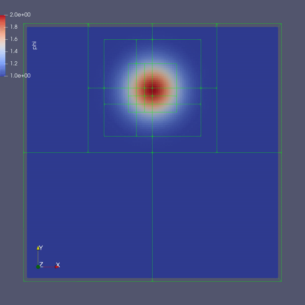
Here is a sample slice through a 3D run with 64x64x8 cells at the coarsest level and three finer levels (4 total levels).
After you run the code you will have a series of plotfiles. To visualize these we will use ParaView 5.8, which has native support for AMReX Grid, Particle, and Embedded Boundary data (in the AMR 101 exercise we only have grid data).
Make a Movie with the ParaView 5.8 Script
To use the ParaView 5.8 python script, simply do the following to generate amr101_3D.gif:
$ make movie3D
If you run the 2D executable, make the 2D movie using:
$ make movie2D
Notes:
-
To delete old plotfiles before a new run, do
rm -rf plt* -
You will need
+ffmpegin your~/.soft.cooleyfile. If you do not already have it, dosoft add +ffmpegand thenresoftto load it. -
You can do
realpath amr101_3D.gifto get the movie’s path on Cooley and then copy it to your local machine by doingscp [username]@cooley.alcf.anl.gov:[path-to-gif] .
Using ParaView 5.8 Manually
To do the same thing with ParaView 5.8 manually (if, e.g. you have the plotfiles on your local machine and want to experiment or if you connected ParaView 5.8 in client-server mode to Cooley):
1. Start Paraview 5.8
2. File --> Open ... and select the collection of directories named "plt.." --> [OK]
3. From the "Open Data With..." dialog that pops up, select "AMReX/BoxLib Grid Reader" --> [OK]
4. Check the "phi" box in the "Cell Array Status" menu that appears
5. Click green Apply button
6. Click on the "slice" icon -- three to the right of the calculator
   This will create "Slice 1" in the Pipeline Browser which will be highlighted.
7. Click on "Z Normal"
8. Unclick the "Show Plane" button
9. Click green Apply button
10. Change the drop-down menu option (above the calculator row) from "vtkBlockColors" to "phi"
You are now ready to play the movie! See the “VCR-like” controls at the top. Click the play button.
Additional Topics to Explore
-
What happens as you change the max grid size for decomposition?
-
What happens as you change the refinement criteria (i.e. use different values of \(\phi\))? (You can edit these in inputs)
Example: “AMR102: Advection of Particles Around Obstacles”
What Features Are We Using
- Mesh data with EB
- Linear solvers (multigrid)
- Particle-Mesh interpolation
The Problem
Challenge:
Recall our previous problem of the drop of dye in a thin incompressible fluid that is spinning clock-wise then counter-clockwise with a prescribed motion.
Now instead of advecting the dye as a scalar quantity defined on the mesh (the continuum representation), we define the dye as a collection of particles that are advected by the fluid velocity.
Again the fluid is thin enough that we can model this as two-dimensional motion; again we have the option of solving in a 2D or 3D computational domain.
To make things even more interesting, there is now an object in the flow, in this case a cylinder. It would be very difficult to analytically specify the flow field around the object, so instead we project the velocity field so that the resulting field represents incompressible flow around the object.
Projecting the Velocity for Incompressible Flow around the Cylinder
Mathematically, projecting the specified velocity field means solving \[\nabla \cdot (\beta \nabla \xi) = \nabla \cdot \bf{u^{spec}}\]
and setting \[\bf{u} = \bf{u^{spec}} - \beta \nabla \xi\]
To solve this variable coefficient Poisson equation, we use the native AMReX geometric multigrid solver. In our case $\beta = 1 / \rho = 1$ since we are assuming constant density $\rho.$
Note that for this example we are solving everything at a single level for convenience, but linear solvers, EB and particles all have full multi-level functionality.
In each timestep we compute the projected velocity field, advect the particles with this velocity, then interpolate the particles onto the mesh to determine \(\phi(x,y,z)\).
Particle-In-Cell Algorithm for Advecting \(\phi\)
We achieve conservation by interpreting the scalar \(\phi\) as the number density of physical dye particles in the fluid, and we represent these physical particles by “computational” particles \(p\). Each particle \(p\) stores a weight \(w_p\) equal to the number of physical dye particles it represents.
This allows us to define particle-mesh interpolation that converts \(\phi(x,y,z)\) to a set of particles with weights \(w_p\). First, we interpolate \(\phi(x,y,z)\) to \(\phi_p\) at each particle location by calculating: \[\phi_p = \sum_i \sum_j \sum_k S_x \cdot S_y \cdot S_z \cdot \phi(i,j,k)\]
where in the above, \(S_{x,y,z}\) are called shape factors, determined by the particle-in-cell interpolation scheme we wish to use.
The simplest interpolation is nearest grid point (NGP), where \(S_{x,y,z} = 1\) if the particle \(p\) is within cell \((i,j,k)\) and \(S_{x,y,z} = 0\) otherwise. An alternative is linear interpolation called cloud-in-cell (CIC), where the shape factors are determined by volume-weighting the particle’s contribution to/from the nearest 8 cells (in 3D).
Once we have interpolated \(\phi(x,y,z)\) to the particle to get \(\phi_p\), we scale it by the volume per particle to get the number of physical dye particles that our computational particle represents. Here, \(n_{ppc}\) is the number of computational particles per cell. \[w_p = \phi_p \cdot \dfrac{dx dy dz}{n_{ppc}}\]
To go back from the particle representation to the grid representation, we reverse this procedure by summing up the number of physical dye particles in each grid cell and dividing by the grid cell volume. This recovers the number density \(\phi(x,y,z)\). \[\phi(i,j,k) = \dfrac{1}{dx dy dz} \cdot \sum_p S_x \cdot S_y \cdot S_z \cdot w_p\]
This approach is the basis for Particle-In-Cell (PIC) methods in a variety of fields, and in this tutorial you can experiment with the number of particles per cell and interpolation scheme to see how well you can resolve the dye advection.
Running the code
cd track-5-numerical/amrex/AMReX_Amr102/Exec
In this directory you’ll see
main2d.gnu.MPI.ex -- the 2D executable -- this has been built with MPI

main3d.gnu.MPI.ex -- the 3D executable -- this has been built with MPI

inputs -- an inputs file for both 2D and 3D
As before, to run the 3D code in serial:
./main3d.gnu.MPI.ex inputs
To run in parallel, for example on 4 ranks:
mpiexec -n 4 ./main3d.gnu.MPI.ex inputs
Similar to the last example, the following parameters can be set at run-time – these are currently set in the inputs file.
stop_time =  2.0                         # the final time (if we have not exceeded number of steps)
max_step  = 200                          # the maximum number of steps (if we have not exceeded stop_time)

n_cell = 64                              # number of cells in x- and y-directions; z-dir has 1/8 n_cell (if 3D)

max_grid_size = 32                       # the maximum number of cells in any direction in a single grid

plot_int = 10                            # frequency of writing plotfiles
The size, orientation and location of the cylinder are specified in the inputs file as well:
cylinder.direction = 2                  # cylinder axis aligns with z-axis
cylinder.radius    = 0.1                # cylinder radius
cylinder.center    = 0.7 0.5 0.5        # location of cylinder center (in domain that is unit box in xy plane)

cylinder.internal_flow = false          # we are computing flow around the cylinder, not inside it
Here you can play around with changing the size and location of the cylinder.
The number of particles per cell and particle-mesh interpolation type are also specified in the inputs file:
n_ppc = 100                              # number of particles per cell for representing the fluid

pic_interpolation = 1                    # Particle In Cell interpolation scheme:
                                         # 0 = Nearest Grid Point
                                         # 1 = Cloud In Cell
You can vary the number of particles per cell and interpolation to see how they influence the smoothness of the phi field.
Questions to answer:
1. How does the solution in the absence of the cylinder compare to our previous solution (where phi was advected
   as a mesh variable)?

2. Note that at the very end we print the time spent creating the geometrical information.
   How does this compare to the total run time?

3. Go back and run the AMR101 example with the same size box and amr.max_level = 1.  How does
   the total run time of the AMR101 code compare with the AMR102 code for 200 steps?
   What probably accounts for the difference?

4. Note that for the purposes of visualization, we deposited the particle weights onto the grid.
   Was phi conserved using this approach?
Visualizing the Results
Make a Movie with the ParaView 5.8 Script
To use the ParaView 5.8 python script, simply do the following to generate amr102_3D.gif:
$ make movie3D
If you run the 2D executable, make the 2D movie using:
$ make movie2D
Notes:
-
To delete old plotfiles before a new run, do
rm -rf plt* -
You will need
+ffmpegin your~/.soft.cooleyfile. If you do not already have it, dosoft add +ffmpegand thenresoftto load it. -
You can do
realpath amr102_3D.gifto get the movie’s path on Cooley and then copy it to your local machine by doingscp [username]@cooley.alcf.anl.gov:[path-to-gif] .
Using ParaView 5.8 Manually
To do the same thing with ParaView 5.8 manually (if, e.g. you have the plotfiles on your local machine and want to experiment or if you connected ParaView 5.8 in client-server mode to Cooley):
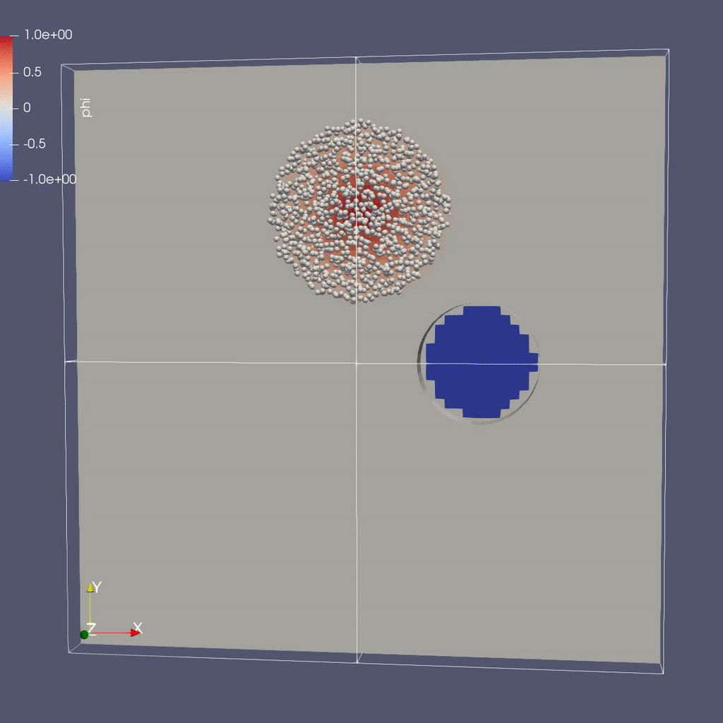
There are three types of data from the simulation that we want to load:
- the mesh data, which includes the interpolated phi field, velocity field and the processor ID
- the EB representation of the cylinder
- the particle locations and weights
To load the mesh data, follow steps 1-10 for plotting \(\phi\) in the AMR 101 tutorial, then continue as below to add the EB representation of the cylinder and the particle data.
Instructions to visualize the EB representation of the cylinder:
1. File --> Open ... select "eb.pvtp" (highlight it then click OK)
2. Click green Apply button
You should see 1 cylinder with its axis in the z-direction.
Now to load the particles:
1. File --> Open ... and select the collection of directories named "plt.." --> [OK]
2. From the "Open Data With..." dialog that pops up, this time select "AMReX/BoxLib Particles Reader" --> [OK]
8. Click green Apply button to read in the particle data
3. Click the "glyph" button (6 to the right of the calculator)
4. Under "Glyph Source" select "Sphere" instead of "Arrow"
6. Under "Scale" set "Scale Factor" to 0.01
7. Under "Masking" change "Glyph Mode" from "Uniform Spatial Distribution" to Every Nth Point
8. Under "Masking", set the stride to 100. The default inputs use 100 particles per cell, which is quite a lot of particles in 3D, so we only plot 1 out of every 100 particles.
9. Change the drop-down menu option (above the calculator row) from "Solid Color" to "real_comp3" to color the particles by their weights.
10.  Click green Apply button
You are now ready to play the movie! See the “VCR-like” controls at the top. Click the play button.
Example: AMReX-Pachinko
What Features Are We Using
- EB for obstacles
- Particle-obstacle and particle-wall collisions
The Problem
Have you ever played pachinko?
A pachinko machine is like a vertical pinball machine.
Balls are released at the top of the “playing field”, and bounce off obstacles as they fall.
The object of the game is to “capture” as many balls as possible.
In the AMReX-Pachinko game you can release as many particles as you like at the top of the domain, and the balls will freeze when they hit the bottom so you can see where they landed.
Your goal here is to see if you can cover the floor of the pachinko machine.
(Note that this is not completely realistic – the balls here don’t feel each other so they can overlap.)
Running the Code
cd track-5-numerical/amrex/AMReX_EB_Pachinko
In this directory you’ll see
main3d.gnu.MPI.ex    -- the executable -- this has been built with MPI

inputs_3d            -- domain size, size of grids, how many time steps, which obstacles...

initial_particles_3d -- initial particle locations  (this name is given in the inputs_3d file)
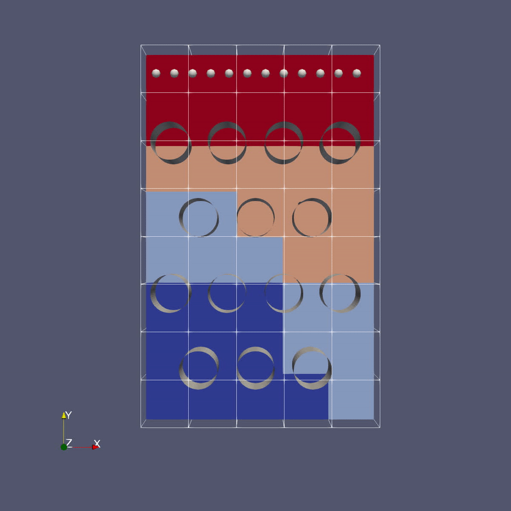
In this example there is no fluid (or other variable) stored on the mesh but we still sort the particles according to our spatial decomposition of the domain. If we run in parallel with 4 processors, we see the domain decomposition below – this results from using a z-order space-filling curve with the number of cells per grid as the cost function.
For now we freeze the obstacles (although if you look in the code it’s not hard to figure out how to change them!) but we can change the initial particle locations at run-time by editing the initial_particles_3d file.
To run in serial,
./main3d.gnu.MPI.ex inputs_3d
To run in parallel, for example on 4 ranks:
mpiexec -n 4 ./main3d.gnu.MPI.ex inputs_3d
The following parameters can be set at run-time – these are currently set in the inputs_3d file. In this specific example we use only 4 cells in the z-direction regardless of n_cell.
n_cell = 125                          # number of cells in x-direction; we double this in the y-direction
max_grid_size = 25                    # the maximum number of cells in any direction in a single grid

plot_int = 10                         # frequency of writing plotfiles

particle_file = initial_particles_3d  # name of file where we specify the input positions of the particles

time_step = 0.001                     # we take a fixed time step of this size

max_time  = 3.0                       # the final time (if max_time < max_steps * time_step)
max_steps = 100000                    # the maximum number of steps (if max_steps * time_step < max_time))
You can also set values on the command line; for example,
mpiexec -n 4 ./main3d.gnu.MPI.ex inputs_3d particle_file=my_file
will read the particles from a file called “my_file”
The output from your run should look something like this:
********************************************************************
 Let's advect the particles ...
   We'll print a dot every 10 time steps.
********************************************************************

.............................................................................................................................................................................................................................................................................................................

********************************************************************
We've finished moving the particles to time 3
That took 1.145916707 seconds.
********************************************************************
Visualizing the Results
Again we’ll use Paraview 5.8 to visualize the results.
As before, to use the Paraview python script, simply do:
$ make movie
(You will need +ffmpeg in your .soft.cooley file)
Remember there are three types of data from the simulation that we want to load:
- the EB representation of the cylinders
- the mesh data, which includes just the processor ID for each grid
- the particle motion
Because the EB data and mesh data don’t change, we load these separately from the particles.
Instructions to visualize the EB representation of the cylinders:
1. Start Paraview 5.8
2. File --> Open ... select "eb.pvtp" (highlight it then click OK)
3. Click green Apply button
You should see cylinders with their axes in the z-direction.
Now to add the mesh field:
1. File --> Open ... and this time select only the directory named "plt00000" --> [OK]
2. From the "Open Data With..." dialog that pops up, select "AMReX/BoxLib Grid Reader" --> [OK]
3. Check the "proc" and "vfrac" boxes in the "Cell Array Status" menu that appears
4. Click green Apply button
5. Click on the "slice" icon -- three to the right of the calculator
   This will create "Slice 1" in the Pipeline Browser which will be highlighted.
6. Click on "Z Normal"
7. Unclick the "Show Plane" button
8. Click green Apply button
9. Change the drop-down menu option (above the calculator row) from "vtkBlockColors" to "proc"
Now to load the particles:
1. File --> Open ... and select the collection of directories named "plt.." --> [OK]
2. From the "Open Data With..." dialog that pops up, this time select "AMReX/BoxLib Particles Reader" --> [OK]
8. Click green Apply button to read in the particle data
3. Click the "glyph" button (6 to the right of the calculator)
4. Under "Glyph Source" select "Sphere" instead of "Arrow"
6. Under "Scale" set "Scale Factor" to 0.05
7. Under "Masking" change "Glyph Mode" from "Uniform Spatial Distribution" to "All Points"
8. Click green Apply button
You are now ready to play the movie! See the “VCR-like” controls at the top. Click the play button.
For fun: if you want to color the particles, make sure “Glyph1” is highlighted, then change the drop-down menu option (above the calculator row) from “vtkBlockColors” to “cpu” – if you have run with 4 processes then you will see the particles displayed with different colors.
Further Reading
Download AMReX from github here.
Look at the AMReX documentation/tutorials here
Read the Journal of Open Source Software (JOSS) paper here