The Multidimensional Rosenbrock Problem
Numerical Optimization with PETSc/TAO
At a Glance
| Questions | Objectives | Key Points |
| 1. What is optimization? | Understand the basic principles | Optimization seeks the inputs of a function that minimizes it |
| 2. Why use gradient-based methods? | Learn about trade-offs in algorithm choice | Gradient-based methods find local minima with the fewest number of function evaluations |
| 3. How can we compute gradients? | Evaluate different sensitivity analysis methods | Applications should provide analytical gradients whenever they can |
| 4. How to solve constrained problems? | Introduce constraints to the optimization problem | Constraints can change the solution or introduce new local minima |
Note: To run the application in this lesson
cd track-5-numerical/numerical_optimization_tao
make multidim_rosenbrock
./multidim_rosenbrock -tao_monitor
Introduction to Optimization
Optimization algorithms seek to find the input variables or parameters (referred to as “control”, “design” or “optimization” variables) that minimize (or maximize) a function of interest. \[\underset{p}{\text{minimize}} \quad f(p),\]
where \(p \in \mathbb{R}^n\) are the optimization variables and \(f(p): \mathbb{R}^{n} \rightarrow \mathbb{R}\) is the objective function. In this lesson, we focus on gradient-based optimization methods – methods that utilize information about the sensitivity of the objective function with respect to its inputs.
Solutions to this problem are found where the gradient of the objective function is zero, \(\nabla_p f(p) = 0\). However, this is only a necessary but not sufficient condition for optimality given that other stationary points (e.g., maxima) also satisfy this condition.
Sequential Quadratic Programming (SQP)
To find local minima for the above problems, we replace the original problem with a sequence of quadratic subproblems, \[\underset{d}{\text{minimize}} \quad f_k + d^Tg_k + \frac{1}{2}d^TH_kd^T,\]
where \(g_k = \nabla_p f(p_k)\) is the gradient, \(H_k = \nabla_p^2 f(p_k)\) is the Hessian, \(d \in \mathbb{R}^n\) is the search direction, and the \(k\) subscript denotes evaluation at the iterate \(p_k\). The exact solution to this quadratic subproblem is the inversion of the Hessian onto the negative gradient, \(d = -H_k^{-1} g_k\). This can also be viewed as the application of the Newton root-finding method to the system of nonlinear equations defined by the optimality condition \(\nabla_p f(p) = 0\).
In order to avoid non-minimum stationary points, we also seek to find a step length \(\alpha\) that approximately minimizes the objective function along the line defined by the search direction, \[\underset{\alpha}{\text{minimize}} \quad \Phi(\alpha) = f(p_k + \alpha d).\]
This scalar minimization problem is called a “line search”, and is categorized as a “globalization” method because it helps maintain consistency between the local quadratic model and the global nonlinear function.
The SQP class of algorithms can be summarized with the pseudocode:
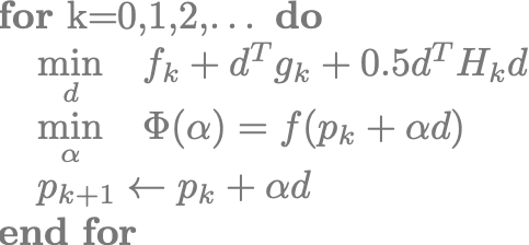
In this approach, different approximations to the search direction solution yield different members of the SQP family:
- Truncated Newton: \(d = -H_k^{-1} g_k\) with Hessian inverted iteratively (e.g., Krylov methods) using dynamic tolerances
- Quasi-Newton: \(d = -B_k g_k\) where \(B_k \approx H_k^{-1}\) with low-rank updates based on the Secant condition
- Conjugate Gradient: \(d_k = -g_k + \beta d_{k-1}\) with \(\beta\) defining different CG update formulas
- Gradient Descent: \(d = g_k\) with Hessian replaced with the identity matrix
Truncated Newton is considered a second-order method because it utilizes full second-order derivative information in the solution of the search direction. Meanwhile, Gradient Descent and Conjugate Gradient methods are clear first-order methods as they only use the gradient of the objective. The Quasi-Newton method, although technically a first-order method, typically exhibits performance closer to Newton’s method by utilizing a Secant approximation to estimate second-order information.
Notes on PDE-constrained Optimization (Click to expand!)
Oftentimes we are interested in solving optimization problems where the evaluation of the objective function depends on the solution of a partial-differential-equation (PDE). These problems are represented in the most general case by \[\underset{p, u}{\text{minimize}} \quad f(p, u) \quad \text{subject to} \quad R(p, u) = 0,\]
where \(u \in \mathbb{R}^m\) are the state or solution variables for the PDE and \(R: \mathbb{R}^{n+m} \rightarrow \mathbb{R}^m\) are the state equations (e.g., discretized PDE residual).
A common and convenient way to recast this problem is to represent the state variables as implicit functions of the optimization variables, \[\underset{p}{\text{minimize}} \quad f(p, u(p)).\]
This eliminates the PDE constraint, converting the problem to an unconstrained version that can be solved by many popular unconstrained optimization algorithms. This comes at the cost of performing a complete PDE solution for every evaluation of the objective function, as well as an adjoint solution to efficiently compute gradients.
For more detail on PDE-constrained optimization, please refer to the “Boundary Control with PETSc/TAO and AMReX” lecture from ATPESC 2019.
Sensitivity Analysis
Sequential Quadratic Programming is a gradient-based approach – i.e., it uses information about the sensitivity of the objective function output to changes in the input (optimization) parameters to iteratively search for the nearest local minimum. In order to use SQP algorithms, the applications must, at minimum, provide first-order derivative information.
In the broadest sense, there are two generalized ways to compute gradients.
Numerical Differentiation approximates the derivative of a function using numerical methods. In the current lecture, we will evaluate the finite difference (FD) method and specifically use the forward difference formulation given by \[\frac{df}{dp_i} = \frac{f(p + he_i) + f(p)}{h} + \mathcal{O}(h) \quad \forall \; i = 1, 2, \dots, N,\]
where \(h\) is the finite perturbation, \(e_i\) is the standard basis vector for the \(i^{th}\) coordinate, and \(\mathcal{O}(h)\) is truncation error for the approximation.
The FD method allows us to compute the gradient for any function easily, using only the function output, without requiring information about the function itself. However, computing each element of the gradient requires a separate function evaluation, causing the computational cost of the method to scale up rapidly with increasing problem sizes.
Furthermore, the FD method also presents a step size dilemma in choosing the numerical magnitude of the perturbation \(h\). The step size must be chosen sufficiently small to minimize truncation error, but also sufficiently large to ensure that subtractive cancellation error does not dominate. Since this cancellation error is problem-dependent, the ideal value of \(h\) differs for each application and may leave the user no choice but to accept the presence of a large error in the gradient.
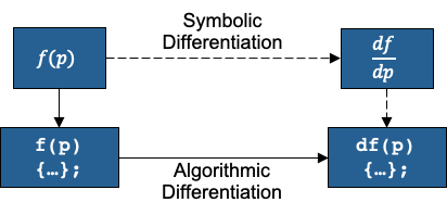
Analytical Differentiation computes the exact derivative by generating a stand-alone mathematical or algorithmic expression for the gradient.
For simpler problems with objective functions that have human-readable closed-form expressions, this approach can be thought of as manually differentiating the expression on paper and implementing a dedicated subroutine to evaluate it. Although the hands-on example problem below is implemented with this approach, it is not suitable for most real-world applications. Practical problems in many scientific disciplines are too complex to be differentiated by hand.
For problems where the objective function depends on a complex subroutine (e.g., the discretized residual for a partial differential equation), algorithmic or automatic differentiation (AD) applies the chain rule to the sequence of elementary operations performed by the function. This is typically done with an AD tool that transforms the source code to generate a new subroutine for the derivative before compile time, or an AD library that overloads the elementary operations in the source code at compile time to generate compiled code for the derivative.
This approach produces accurate gradients at a computational cost that is largely insensitive to the size of the optimization problem. However, the FD methods remain an easy alternative for rapid prototyping and testing, especially when the problem size is small and objective function evaluations are not expensive.
Below is an incomplete list of AD tools that may be useful to your application:
- ADIC (ANSI C) – Argonne National Laboratory
- ADIFOR (Fortran77) – Argonne National Laboratory
- OpenAD (Fortran77/Fortran95/C/C++) – Argonne National Laboratory
- Sacado (C/C++) – Sandia National Laboratory
- ForwardDiff.jl (Julia)
- JAX (Python)
- TOMLAB/MAD (MATLAB)
Using TAO
Toolkit for Advanced Optimization (TAO) is a package of optimization algorithms and tools developed at Argonne National Laboratory and distributed with the Portable Extensible Toolkit for Scientific Computing (PETSc) library. TAO is primarily intended for continuous gradient-based optimization and supports PDE-constrained problems using the reduced-space formulation.
Below is a TAO main file template that can be adapted to any gradient-based optimization problem:
#include "petsc.h"

typedef struct {
  int n; /* number of optimization variables */
} AppCtx;

PetscErrorCode FormFunction(Tao tao, Vec P, PetscReal *fcn, void *ptr)
{
  PetscErrorCode ierr;
  AppCtx *user = (AppCtx*)ptr;

  /* Compute the objective function at point P and store in fcn */

  return 0;
}

PetscErrorCode FormGradient(Tao tao, Vec P, Vec G, void *ptr)
{
  PetscErrorCode ierr;
  AppCtx *user = (AppCtx*)ptr;

  /* Compute the gradient at point P and store in vector G */

  return 0;
}

PetscErrorCode FormHessian(Tao tao, Vec P, Mat H, Mat Hpre, void *ptr)
{
  PetscErrorCode ierr;
  AppCtx *user = (AppCtx*)ptr;

  /* Compute the Hessian at point P and store in matrix H */
  /* Note: Hpre is an OPTIONAL preconditioner for inverting the Hessian */

  return 0;
}

int main(int argc, char *argv[])
{
  PetscErrorCode ierr;
  AppCtx user;
  Tao tao;
  Vec X;
  Mat H;

  /* Initialize the PETSc library */
  ierr = PetscInitialize( &argc, &argv, (char *)0, (char *)0);if (ierr) return ierr;

  /* Create solution vector and Hessian matrix */
  ierr = VecCreate(PETSC_COMM_WORLD, &X);CHKERRQ(ierr);
  ierr = VecSetSizes(X, PETSC_DECIDE, user.n);CHKERRQ(ierr);
  ierr = VecSet(X, 0.0);CHKERRQ(ierr);
  ierr = MatCreate(PETSC_COMM_WORLD, &H);CHKERRQ(ierr);
  ierr = MatSetSizes(H, PETSC_DECIDE, PETSC_DECIDE, user.n, user.n);CHKERRQ(ierr);
  ierr = MatSetUp(H);CHKERRQ(ierr);

  /* Create Tao solver and configure */
  ierr = TaoCreate(PETSC_COMM_WORLD, &tao);CHKERRQ(ierr);
  ierr = TaoSetType(tao, TAOBQNLS);CHKERRQ(ierr);
  ierr = TaoSetInitialVector(tao, X);CHKERRQ(ierr);
  ierr = TaoSetObjectiveRoutine(tao, FormFunction, &user);CHKERRQ(ierr);
  ierr = TaoSetGradientRoutine(tao, FormGradient, &user);CHKERRQ(ierr);
  ierr = TaoSetHessianRoutine(tao )
  ierr = TaoSetFromOptions(tao);CHKERRQ(ierr);

  /* Trigger the solution */
  ierr = TaoSolve(tao);CHKERRQ(ierr);

  /* Clean up PETSc objects and finalize */
  ierr = VecDestroy(&X);CHKERRQ(ierr);
  ierr = MatDestroy(&H);CHKERQ(ierr);
  ierr = TaoDestroy(&tao);CHKERRQ(ierr);
  ierr = PetscFinalize();

  return 0;
}
TAO calls the user-provided FormFunction(), FormGradient() and FormHessian() routine whenever the
optimization algorithm needs to evaluate the objective, its gradient and Hessian. The AppCtx structure contains
any data the user has to preserve and propagate through for these computations.
Applications where it is more efficient to evaluate the objective function together with the gradient can use
an alternative TaoSetObjectiveAndGradientRoutine() interface to provide TAO a single FormFunctionGradient()
callback that evaluates both at the same time.
TAO implements several bound-constrained algorithm types that also solve unconstrained problems when there are no
bounds defined in the problem setup. Algorithm types can be changed either via the TaoSetType() interface using the
solver names given in the first column below, or changed at runtume with the option flag -tao_type <solver> using the
string arguments given in the second column.
| Solver Type | Option Flag | Description |
TAOBNLS
| bnls
| Bound-constrained Newton Line Search |
TAOBNTR
| bntr
| Bound-constrained Newton Trust Region |
TAOBQNLS
| bqnls
| Bound-constrained Quasi-Newton Line Search |
TAOBNCG
| bncg
| Bound-constrained Nonlinear Conjugate Gradient |
The TAO solution can also be configured with additional runtime flags and corresponding code interfaces shown below.
| Option Flag | Code API | Description |
-tao_monitor
| TaoSetMonitor() with TaoMonitorDefault()
| Enable the iteration monitor for the solution |
-tao_view
| TaoView()
| Display useful information about the solution after completion |
-tao_max_it <integer>
| TaoSetMaximumIterations()
| Change the maximum iteration limit |
-tao_max_funcs <integer>
| TaoSetMaximumFunctionEvaluations()
| Change the maximum number of function evaluations |
-tao_gatol <float>
| TaoSetTolerances()
| Change the absolute convergence tolerance |
-tao_test_gradient
| TaoTestGradient()
| Validate the analytical gradient with finite differences at every iteration |
-tao_test_hessian
| TaoTestHessian()
| Validate the analytical Hessian with finite differences at every iteration |
Defining Constraints(Click to expand!)
The discussion so far has focused exclusively on unconstrained problems even though the TAO solvers listed above are all capable of solving bound-constrained problems. Bounds, which are also sometimes called “box” constraints, are scalar limits placed on the optimization variables, such that \[\begin{align} \underset{p}{\text{minimize}} &\quad f(p) \\ \text{subject to} &\quad p_l \leq p \leq p_u \end{align}\]
where \(p_l\) and \(p_u\) are the lower and upper bound vectors, respectively. In optimization problems solved with TAO, users can set the bounds with the following workflow:
/* Duplicate from solution vector and set bounds */
ierr = VecDuplicate(X, &XL);CHKERRQ(ierr);
ierr = VecSet(XL, PETSC_NINFINITY);CHKERRQ(ierr);
ierr = VecDuplicate(X, &XU);CHKERRQ(ierr);
ierr = VecSet(XU, 0.0);CHKERRQ(ierr);
ierr = TaoSetVariableBounds(tao, XL, XU);CHKERRQ(ierr);
In this particular example, the lower bound is set to negative-infinity which designates it as “unbounded”, and the
upper bound is zero, thus forcing the solver to produce zero or negative solutions only. For positive solutions, the
lower bound would be set to 0 while the upper bound would be set to PETSC_INFINITY. Furthermore, the bounds can also
be adjusted differently for individual optimization variables using VecSetValue(xl, i, val, INSERT_VALUES) where i
is the index of the variable and val is the boundary value.
In addition to bound-constrained methods, TAO also implements an Augmented Lagrangian Method of Multipliers (TAOALMM)
for generally constrained optimization problems of the form:
\[\begin{align}
\underset{p}{\text{minimize}} &\quad f(p) \\
\text{subject to} &\quad c_e(p) = 0 \\
&\quad c_i(p) \leq 0 \\
&\quad p_l \leq p \leq p_u
\end{align}\]
TAOALMM converts this inequality constraints to equality constraints using an interior-point formulation, and then
converts the equality constrained problem into a sequence of unconstrained or bound-constrained problems using the
augmented Lagrangian method. The unconstrained/bound-constrained subproblems are solved by one of the existing
bound-constrained TAO solvers.
TAO requires equality and inequality constraints to be defined as function callbacks, separately for the constraint vector and its Jacobian (matrix of sensitivities).
PetscErrorCode FormEqualityConstraints(Tao tao, Vec P, Vec CE, void* ptr)
{
  PetscErrorCode ierr;
  AppCtx *user = (AppCtx*)ptr;

  /* Compute the vector of equality constraints CE at solution P */

  return 0;
}

PetscErrorCode FormEqualityJacobian(Tao tao, Vec P, Mat AE, Mat AEpre, void* ptr)
{
  PetscErrorCode ierr;
  AppCtx *user = (AppCtx*)ptr;

  /* Compute the equality constraint Jacobian matrix AE at solution P */
  /* NOTE: AEpre represents a "pseudoinverse" of AE but is ignored in most applications */

  return 0;
}

PetscErrorCode FormInqualityConstraints(Tao tao, Vec P, Vec CI, void* ptr)
{
  PetscErrorCode ierr;
  AppCtx *user = (AppCtx*)ptr;

  /* Compute the vector of equality constraints CI at solution P */

  return 0;
}

PetscErrorCode FormEqualityJacobian(Tao tao, Vec P, Mat AI, Mat AIpre, void* ptr)
{
  PetscErrorCode ierr;
  AppCtx *user = (AppCtx*)ptr;

  /* Compute the inequality constraint Jacobian matrix AI at solution P */
  /* NOTE: AIpre represents a "pseudoinverse" of AI but is ignored in most applications */

  return 0;
}

int main(int argc, char *argv[])
{
  /*
    problem code
  */

  /* Equality constraints */
  ierr = VecCreate(PETSC_COMM_WORLD, &CE);CHKERRQ(ierr);
  ierr = VecSetSizes(CE, PETSC_DECIDE, user.nce);CHKERRQ(ierr);
  ierr = TaoSetEqualityConstraintsRoutine(tao, CE, FormEqualityConstraints, &user);CHKERRQ(ierr);
  ierr = MatCreate(PETSC_COMM_WORLD, &AE);CHKERRQ(ierr);
  ierr = MatSetSizes(AE, PETSC_DECIDE, PETSC_DECIDE, user.nce, user.n);CHKERRQ(ierr);
  ierr = MatSetUp(AE);CHKERRQ(ierr);
  ierr = TaoSetJacobianEqualityRoutine(tao, AE, AE, FormEqualityJacobian, &user);CHKERRQ(ierr);

  /* Inquality constraints */
  ierr = VecCreate(PETSC_COMM_WORLD, &CI);CHKERRQ(ierr);
  ierr = VecSetSizes(CI, PETSC_DECIDE, user.nci);CHKERRQ(ierr);
  ierr = TaoSetEqualityConstraintsRoutine(tao, CI, FormInequalityConstraints, &user);CHKERRQ(ierr);
  ierr = MatCreate(PETSC_COMM_WORLD, &AI);CHKERRQ(ierr);
  ierr = MatSetSizes(AI, PETSC_DECIDE, PETSC_DECIDE, user.nci, user.n);CHKERRQ(ierr);
  ierr = MatSetUp(AI);CHKERRQ(ierr);
  ierr = TaoSetJacobianEqualityRoutine(tao, AI, AI, FormEqualityJacobian, &user);CHKERRQ(ierr);

  /*
    more problem code...
  */
  return 0;
}
Example Problem: Multidimensional Rosenbrock
|
|
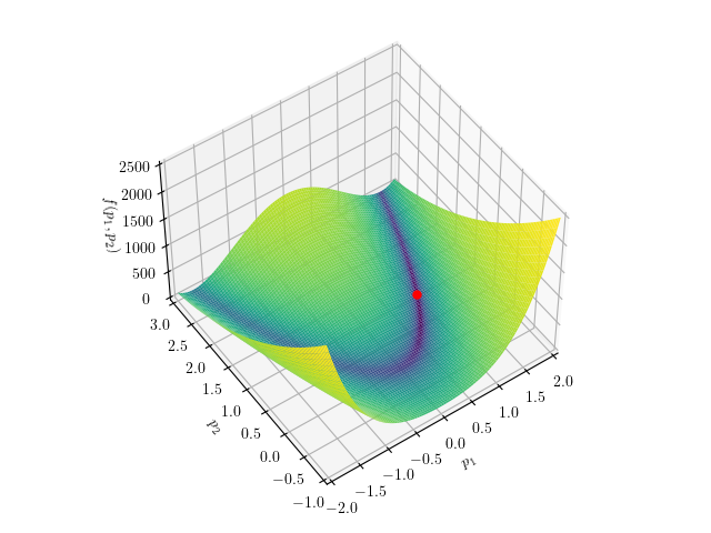
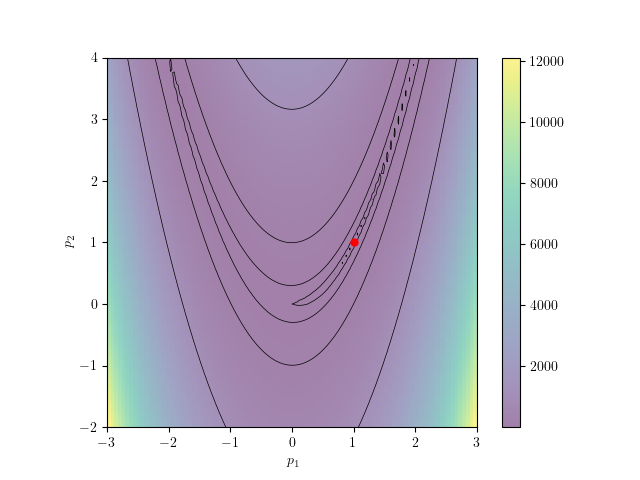
The Rosenbrock function, also called a “banana function”, is a canonical nonconvex test problem created by Howard H. Rosenbrock in 1960 and used extensively to evaluate the performance of optimization algorithms. The original function is defined as \[f(p_1, p_2) = (1 - p_1)^2 + 100(p_2 - p_1^2)^2,\]
with a global minimum at \(f(1, 1)=0\).
In this lecture, we will be using a multidimensional generalization of this problem is given by \[f(p) = f(p_1, p_2, \dots, p_N) = \sum_{i=1}^{N-1} \left[ (1 - p_i)^2 + 100(p_{i+1} - p_i^2)^2 \right],\]
with a global minimum at \(p_i = 1 \; \forall i=1,2,\dots,N\).
Gradient and Hessian Definitions (Click to expand!)
The gradient of the multidimensional Rosenbrock problem is given as \[\begin{align} \frac{df}{dp_1} &= -400p_1(p_2 - p_1^2) -2(1 - p_1), \\ \frac{df}{dp_j} &= 200(p_j - p_{j-1}^2) - 400p_j(p_{j+1} - p_j^2) - 2(1 - p_j) \quad \forall \; j = 2, 3, \dots, N-1, \\ \frac{df}{dp_N} &= 200(p_N - p_{N-1}^2). \end{align}\]
The Hessian is a tridiagonal sparse matrix with nonzero elements given as \[\begin{align} \frac{d^2f}{dp_1^2} &= 1200p_1^2 - 400p_2 + 2, \\ \frac{d^2f}{dp_i dp_{i-1}} &= -400p_{i-1} \quad \forall \; i= 2, 3, \dots, N-1, \\ \frac{d^2f}{dp_i dp_i} &= 202 + 1200p_i^2 - 400p_{i+1} \quad \forall \; i= 2, 3, \dots, N-1, \\ \frac{d^2f}{dp_i dp_{i+1}} &= -400p_i \quad \forall \; i= 2, 3, \dots, N-1, \\ \frac{d^2f}{dp_N^2} &= 200. \end{align}\]
The hands-on example implements the multidimensional Rosenbrock with an analytical gradient and Hessian. However,
TAO also provides TaoDefaultComputeGradient() and TaoDefaultComputeHessian() callbacks that utilize
finite-differencing to generate the required sensitivities.
Compile and run the source code as below to solve the default two-dimensional case. If running
on a different machine than ALCF Cooley, the PETSC_DIR variable in the makefile must be changed to
reflect the local PETSc/TAO installation.
$ make multidim_rosenbrock
$ ./multidim_rosenbrock -tao_monitor
Output of run (Click to expand!)
  0 TAO,  Function value: 810081.,  Residual: 360468.
  1 TAO,  Function value: 40609.1,  Residual: 44602.6
  2 TAO,  Function value: 18292.1,  Residual: 26530.2
  3 TAO,  Function value: 2740.19,  Residual: 8336.03
  4 TAO,  Function value: 403.632,  Residual: 2847.47
  5 TAO,  Function value: 26.0168,  Residual: 613.641
  6 TAO,  Function value: 5.30456,  Residual: 68.5064
  7 TAO,  Function value: 5.03392,  Residual: 2.16505
  8 TAO,  Function value: 5.03363,  Residual: 0.684219
  9 TAO,  Function value: 5.03338,  Residual: 1.33861
 10 TAO,  Function value: 5.03266,  Residual: 2.50008
 11 TAO,  Function value: 5.02887,  Residual: 6.6995
 12 TAO,  Function value: 5.02077,  Residual: 12.1942
 13 TAO,  Function value: 4.9971,  Residual: 21.9372
 14 TAO,  Function value: 4.92945,  Residual: 37.3688
 15 TAO,  Function value: 3.26493,  Residual: 42.1352
 16 TAO,  Function value: 3.2562,  Residual: 32.3228
 17 TAO,  Function value: 3.10607,  Residual: 28.7837
 18 TAO,  Function value: 2.7978,  Residual: 33.9724
 19 TAO,  Function value: 2.51192,  Residual: 72.1079
 20 TAO,  Function value: 2.05028,  Residual: 2.87221
 21 TAO,  Function value: 1.72363,  Residual: 17.2465
 22 TAO,  Function value: 1.6214,  Residual: 31.1365
 23 TAO,  Function value: 1.46398,  Residual: 34.627
 24 TAO,  Function value: 1.14514,  Residual: 21.2909
 25 TAO,  Function value: 0.912949,  Residual: 15.3829
 26 TAO,  Function value: 0.66683,  Residual: 9.01563
 27 TAO,  Function value: 0.583865,  Residual: 18.3828
 28 TAO,  Function value: 0.372904,  Residual: 15.1225
 29 TAO,  Function value: 0.360527,  Residual: 16.3198
 30 TAO,  Function value: 0.204402,  Residual: 14.3335
 31 TAO,  Function value: 0.191564,  Residual: 0.750976
 32 TAO,  Function value: 0.150045,  Residual: 3.79711
 33 TAO,  Function value: 0.127328,  Residual: 8.00461
 34 TAO,  Function value: 0.106561,  Residual: 8.3052
 35 TAO,  Function value: 0.075763,  Residual: 9.01468
 36 TAO,  Function value: 0.0181941,  Residual: 0.47139
 37 TAO,  Function value: 0.0135709,  Residual: 1.84761
 38 TAO,  Function value: 0.0115372,  Residual: 2.40889
 39 TAO,  Function value: 0.00713039,  Residual: 2.63071
 40 TAO,  Function value: 0.00277352,  Residual: 1.47662
 41 TAO,  Function value: 0.000626325,  Residual: 0.318311
 42 TAO,  Function value: 0.000151588,  Residual: 0.531674
 43 TAO,  Function value: 1.83371e-06,  Residual: 0.0102533
 44 TAO,  Function value: 1.02401e-08,  Residual: 0.00271617
 45 TAO,  Function value: 8.88669e-12,  Residual: 0.000127435
 46 TAO,  Function value: 5.40216e-17,  Residual: 1.70011e-07
 47 TAO,  Function value: 2.17778e-22,  Residual: 1.98976e-10

Solution time: 0.005766

Solution vector:
Vec Object: 1 MPI processes
  type: seq
1.
1.

Objective at solution: 0.000000
In this output, the Residual indicates the L2-norm of the gradient, \(\|g_k\|_2\), at every iteration. The problem
file is configured to terminate the solution when this gradient norm drops below the absolute tolerance of \(10^{-5}\).
The hands-on example can be modified using the following command-line options:
| Option Flag | Description |
-n <integer>
| Change the problem size (default: 2) |
-fd
| Use finite-difference gradients instead of analytical |
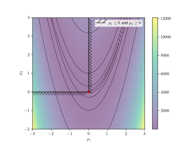
-bound
| Activate bound constraints – 2-D only (default: \(p_1 \leq 0, \; p_2 \geq 0\)) |
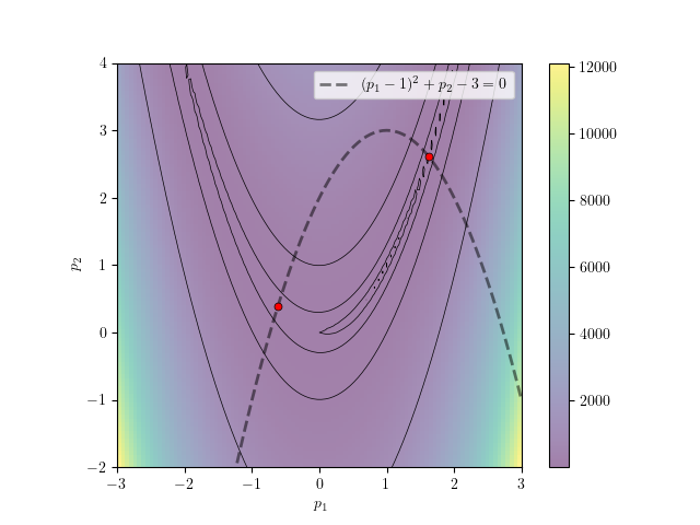
-eq
| Activate equality constraints – 2-D only (default: \((p_1 - 1)^2 + p_2 - 3 = 0\)) |
Hands-on Activities
-
Change the TAO algorithm to nonlinear conjugate gradient method using
-tao_type bncgand to truncated Newton using-tao_type bnls. Compare convergence against the default quasi-Newton method (-tao_type bqnls). - Increase the problem size with the
-n <size>argument (default size is 2) and evaluate its impact on convergence.- Repeat Activity 2 with different TAO algorithms. Do they all exhibit the same scaling?
- Repeat Activity 2 with different TAO algorithms. Do they all exhibit the same scaling?
-
Solve the problem with the finite difference gradient using the
-fdargument. Evaluate convergence and solution time with increasing problem size. - Try running the problem in parallel with
mpiexec -n <# of processes> ./multidim_rosenbrock .... Why does running in parallel slow the solution down at small problem sizes? How large should the problem be to observe a speedup in parallel runs?- Repeat Activity 4 with different TAO algorithms. Are the break-even points in size vs. performance the same?
- Repeat Activity 4 with different TAO algorithms. Are the break-even points in size vs. performance the same?
- Run the problem with
-boundflag to enable \(p_1 \leq 0\) and \(p_2 \geq 0\) constraints.- Change the starting point and evaluate how it affects the convergence. Is there a difference between starting from the feasible versus non-feasible space?
- Repeat Activity 5 with different bound-constrained TAO algorithms.
- Run the problem with
-eqflag to enable the \((p_1 - 1)^2 + p_2 = 3\) constraint.- Change the starting point to \((-1,-1)\) and evaluate whether you recover the same solution as before. If not, why?
- Combine equality constraints with bound constraints and try changing the starting point back to \((10,10)\). Which
solution did you converge to?
- ADVANCED: Change the constraint definition. Come up with constraints that are valid for the multidimensional
Rosenbrock problem.
Notes on Hands-on Activities (Click to expand!)
The original Rosenbrock function is a challenging optimization problem to solve despite its small size. The minimum lies in a banana shaped valley that is easy to find for most methods but difficult to traverse through.
The multidimensional variant presents an additional challenge because the numerical magnitude of the sensitivity terms rapidly scale up with the size of the problem and lead to ill-conditioning in the Hessian. This property causes the convergence of second-order methods to a-typically degrade at particularly large problem sizes.
Similar pathologies present themselves often in practical applications. In many cases, simply adding second-order information does not result in improved ‘‘time-to-solution’’. Even though second-order algorithms such as truncated Newton methods may converge to the specified tolerance in fewer iterations, each iteration may take significantly more time than first-order methods due to the expensive assembly and/or inversion of a Hessian matrix.
The hands-on activities above are intended to reveal these interactions and trade-offs between problem size, algorithm choice, application-specific pathologies, and parallelization.
Notes on Bound Constraints (Click to expand!)
Introducing the bound constraints \(p_1 \leq 0\) and \(p_2 \geq 0\) forces the solution to a new global minimum at \(f(0,0) = 1.0\). This minimum is a trivial solution where the bounds for both optimization variables. are active.
Notes on Equality Constraints (Click to expand!)
The quadratic equality constraint \((p_1 - 1)^2 + p_2 - 3 = 0\) presents two local minima instead of the original global minimum. These two minima lie at \(f(1.62, 2.62)=0.38\) and \(f(-0.62, 0.38)=2.62\). On multi-modal problems such as this, gradient-based optimization methods converge to the local minimum closest to the starting point. In this hands-on example, we start our solution with an initial guess of \((10,10)\) and converge to \(f(1.62, 2.62)=0.38\). A solution that starts at \((-1,-1)\) converges to \(f(-0.62, 0.38)=2.62\) instead.
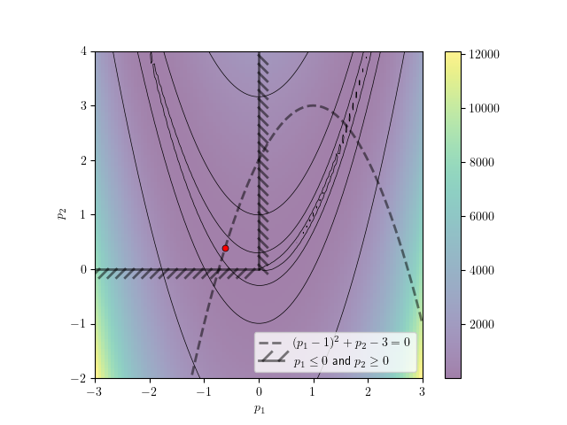
Combining the equality and bound constraints eliminates one of the two local minima and forces the solution to always converge to the now-global minimum at \(f(-0.62, 0.38)=2.62\) regardless of the starting point.
Take-Away Messages
- PETSc/TAO offers parallel optimization algorithms for large-scale problems.
- Applications should provide efficient gradient evaluations for best results (e.g., algorithmic differentiation).
- Second-order optimization methods don’t always achieve faster/better solutions. Sometimes “less is more”.
- When applications provide only function evaluations, PETSc/TAO can automatically compute gradients with finite differencing.
- PETSc/TAO can also use finite differencing to validate application-provided gradients and Hessians.
- Different types of constraints imposed on the problem can change the solution, introduce new local minima, or eliminate existing local minima.
- PETSc/TAO implements methods that can solve problems with both bound, equality and inequality constraints.