Nonlinear Solvers
Nonlinear Solvers with PETSc
At a Glance
| Questions | Objectives | Key Points |
| 1. What are the tradeoffs between exactness and inexactness in Newton methods? | Observe trade-offs between inner and outer iterations as linear solver tolerance is varied | An inexact linear solver may be less robust but can result in significantly faster nonlinear solver |
| 2. What makes a scalable inexact Newton method? | Observe execution time and convergence behavior as mesh spacing is decreased | Newton methods exhibit mesh independent convergence, but need to be combined with scalable linear solvers |
| 3. How and when do nonlinear solvers fail? | Explore limits of nonlinear solvers by systematically increasinging problem nonlinearity | Nonlinear solvers can fail in a variety of ways, and some workarounds exist |
| 4. Can we improve the robustness of Newton’s method by combining it with other solvers? | Explore nonlinear preconditioning for highly nonlinear problems | Nonlinear analogs of ideas from iterative linear solvers can significantly improve nonlinear solvers |
Note: To build the executable used in this lesson do
cd track-5-numerical/nonlinear_solvers_petsc
# The ex19 executable should already exist, but if it needs to be rebuilt, do
make ex19
Introduction
Systems of nonlinear equations \[F(x) = b \quad \mathrm{where} \quad F : \mathbb{R}^N \to \mathbb{R}^N\]
arise in countless settings in computational science. Unlike their linear counterparts, direct methods for general nonlinear systems do not exist. Iterative methods are required!
In this lesson, we will do some hands-on exploration, solving a model nonlinear problem using the nonlinear solvers from the PETSc library. We will focus on variants on Newton’s method, exploring exact vs. inexact Newton methods, Newton-Krylov, and Newton-Krylov-multigrid methods. We will end with some exploration of a topic that is relatively unexplored both theoretically and experimentally: nonlinear preconditioning.
The Problem We Are Solving: the driven cavity CFD benchmark
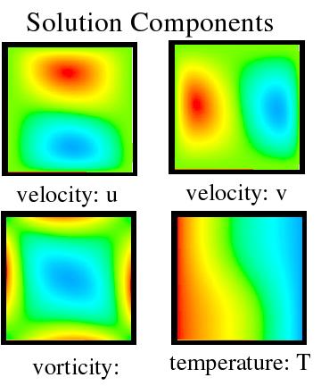
We will use the nonlinear solvers provided by the PETSc Scalable Nonlinear Equation Solvers
(SNES) component to solve the steady-state nonisothermal driven cavity problem as implemented
in SNES example ex19.
This is a classic CFD benchmark that simulates a fluid-filled 2D box with a lid that moves at
constant tangential velocity (probably employing a conveyor belt).
Flow is driven by both the lid motion and buoyancy effects.
Our example uses a velocity-vorticity formulation, in which the governing equations can
be expressed as
\[\begin{align*}
- \Delta U - \partial_y \Omega &= 0 \\
- \Delta V + \partial_x \Omega &= 0 \\
- \Delta \Omega + \nabla \cdot ([U \Omega, V \Omega]) - \mathrm{Gr}\ \partial_x T &= 0 \\
- \Delta T + \mathrm{Pr}\ \nabla \cdot ([U T, V T]) &= 0
\end{align*}\]
where \(U\) and \(V\) are velocities, \(T\) is temperature, \(\Omega\) is vorticity, \(\mathrm{Gr}\) is the Grashof number and \(\mathrm{Pr}\) is the Prandtl number.
Example 1: Initial exploration and understanding PETSc options
Let’s begin by running the ex19 on a single MPI rank with some basic command line options.
./ex19 -snes_monitor -snes_converged_reason -da_grid_x 16 -da_grid_y 16 -da_refine 2 -lidvelocity 100 -grashof 1e2
You should see output similar to
lid velocity = 100., prandtl # = 1., grashof # = 100.
  0 SNES Function norm 7.681163231938e+02
  1 SNES Function norm 6.582880149343e+02
  2 SNES Function norm 5.294044874550e+02
  3 SNES Function norm 3.775102116141e+02
  4 SNES Function norm 3.047226778615e+02
  5 SNES Function norm 2.599983722908e+00
  6 SNES Function norm 9.427314747057e-03
  7 SNES Function norm 5.212213461756e-08
Nonlinear solve converged due to CONVERGED_FNORM_RELATIVE iterations 7
Number of SNES iterations = 7
The table below explains the options we have used:
| Option Flag | Effect |
-snes_monitor
| Show progress of the SNES solver |
-snes_converged_reason
| Print reason for SNES convergence or divergence |
-da_grid_x 16
| Set initial grid points in x direction to 16 |
-da_grid_y 16
| Set initial grid poings in y direction to 16 |
-da_refine 2
| Refine the initial grid 2 times before creation |
-lidvelocity 100
| Set dimensionless velocity of lid to 100 |
-grashof 1e2
| Set Grashof number to 1e2 |
An element of the PETSc design philosphy is extensive runtime customizability.
We can always use -help to enumerate and explain the various command-line options
available to a PETsc executable.
(Note that the help will be tailored to according to the set of options being specified.)
To see the details of how our SNES solver is configured, we can add -snes_view, which will
print information at the end of the run about the SNES object and the underlying KSP
(linear solvers) and PC (preconditioners) objects.
Example -snes_view output
-snes_view outputNonlinear solve converged due to CONVERGED_FNORM_RELATIVE iterations 7
SNES Object: 1 MPI processes
type: newtonls
maximum iterations=50, maximum function evaluations=10000
tolerances: relative=1e-08, absolute=1e-50, solution=1e-08
total number of linear solver iterations=835
total number of function evaluations=11
norm schedule ALWAYS
Jacobian is built using colored finite differences on a DMDA
SNESLineSearch Object: 1 MPI processes
type: bt
interpolation: cubic
alpha=1.000000e-04
maxstep=1.000000e+08, minlambda=1.000000e-12
tolerances: relative=1.000000e-08, absolute=1.000000e-15, lambda=1.000000e-08
maximum iterations=40
KSP Object: 1 MPI processes
type: gmres
restart=30, using Classical (unmodified) Gram-Schmidt Orthogonalization with no iterative refinement
happy breakdown tolerance 1e-30
maximum iterations=10000, initial guess is zero
tolerances: relative=1e-05, absolute=1e-50, divergence=10000.
left preconditioning
using PRECONDITIONED norm type for convergence test
PC Object: 1 MPI processes
type: ilu
out-of-place factorization
0 levels of fill
tolerance for zero pivot 2.22045e-14
matrix ordering: natural
factor fill ratio given 1., needed 1.
Factored matrix follows:
Mat Object: 1 MPI processes
type: seqaij
rows=14884, cols=14884, bs=4
package used to perform factorization: petsc
total: nonzeros=293776, allocated nonzeros=293776
total number of mallocs used during MatSetValues calls=0
using I-node routines: found 3721 nodes, limit used is 5
linear system matrix = precond matrix:
Mat Object: 1 MPI processes
type: seqaij
rows=14884, cols=14884, bs=4
total: nonzeros=293776, allocated nonzeros=293776
total number of mallocs used during MatSetValues calls=0
using I-node routines: found 3721 nodes, limit used is 5
Managing PETSc Options
PETSc offers a very large number of runtime options. All can be set via command line, but can also be set from input files and shell environment variables.
To facilitate readability, we’ll put the command-line arguments common to the remaining
hands-on exercises in the PETSC_OPTIONS environment variable.
export PETSC_OPTIONS="-snes_monitor -snes_converged_reason -lidvelocity 100 -da_grid_x 16 -da_grid_y 16 -ksp_converged_reason -log_view :log.txt"
We’ve added -ksp_converged_reason to see how and when linear solver halts.
We’ve also added -log_view to write the PETSc performance logging info to a file, log.txt.
Such performance logs are full of useful information for understanding the performance of
a PETSc code, but we don’t have time to explore them in this session.
(For those interested, see Chapter 13, “Profiling”, of the
PETSc User Manual.)
Here, we will simply use the performance logs to find the overall wall-clock time via,
which we can quickly find by using the grep utility:
grep Time\ \(sec\): log.txt
(The first number returned is the total run time in seconds.)
IMPORTANT: When you finish these hands-on lessons, be sure to clear your PETSC_OPTIONS environment variable
(do “unset PETSC_OPTIONS”) if you will be doing hands-on exercises in another session.
Otherwise, you may get unexpected behavior if running executables that are linked against PETSc.
Example 2: Exact vs. Inexact Newton
The output from running -snes_view in the previous exercise shows us that PETSc defaults
to an inexact Newton method. To run with exact Newton (and to check the execution time), we
use -pc_type lu, which indicates to the KSP object (which controls the linear solver) that
the underlying preconditioner should be an full LU decomposition:
./ex19 -da_refine 2 -grashof 1e2 -pc_type lu
grep Time\ \(sec\): log.txt
(Remember, the above command assumes that you have set PETSC_OPTIONS as specified in the
preceding section.)
Sample output on my laptop (Dell XPS 13 with Intel Core i7-10710U CPU)
rmills@encke:~/proj/petsc/src/snes/tutorials (master=)$ ./ex19 -da_refine 2 -grashof 1e2 -pc_type lu
lid velocity = 100., prandtl # = 1., grashof # = 100.
  0 SNES Function norm 7.681163231938e+02
  Linear solve converged due to CONVERGED_RTOL iterations 1
  1 SNES Function norm 6.581690463182e+02
  Linear solve converged due to CONVERGED_RTOL iterations 1
  2 SNES Function norm 5.291809327801e+02
  Linear solve converged due to CONVERGED_RTOL iterations 1
  3 SNES Function norm 3.772079270664e+02
  Linear solve converged due to CONVERGED_RTOL iterations 1
  4 SNES Function norm 3.040001036822e+02
  Linear solve converged due to CONVERGED_RTOL iterations 1
  5 SNES Function norm 2.518761157519e+00
  Linear solve converged due to CONVERGED_RTOL iterations 1
  6 SNES Function norm 9.230363584762e-03
  Linear solve converged due to CONVERGED_RTOL iterations 1
  7 SNES Function norm 6.155757710494e-09
Nonlinear solve converged due to CONVERGED_FNORM_RELATIVE iterations 7
Number of SNES iterations = 7
rmills@encke:~/proj/petsc/src/snes/tutorials (master=)$ grep Time\ \(sec\): log.txt
Time (sec):           6.728e-01     1.000   6.728e-01
The work required to solve the inner, linear interation so precisely is likely wasted. Let’s try using the default iterative solver with some different tolerances. Start with
./ex19 -da_refine 2 -grashof 1e2 -ksp_rtol 1e-8
and then try some larger values for relative convergence tolerance, -ksp_rtol.
Try -ksp_rtol 1e-5 (the PETSc default) next, and try increasing it by an order of
magnitude each time.
What happens to the SNES iteration count? When does the SNES solve diverge?
The SNES iteration count is 7 initially, then increases to 8 at a relative tolerance of 1e-3 for the linear solver, and then 10 at a tolerance of 1e-2. The SNES solve diverges when run with a linear solver tolerance of 1e-1.
What yields the shortest execution time?
On my laptop, the loosest tolerance I tried, -ksp_rtol 1e-2, turns out to be fastest, able
to solve the problem in 0.43 seconds. Though it requires more Newton iterations, it performs
far fewer linear solver iterations. Running with the default tolerance of 1e-5 requires
0.60 seconds. A tolerance of 1e-8 is far too high, resulting in many linear solver iterations
and an execution time of over 1.2 seconds.
Using LU factorization turns out to not be too bad for this small problem (around 0.68
seconds), but it is difficult for LU to scale up to large problems.
Example 3: Scaling up the grid size and running in parallel
Let’s explore what happens as we scale up the grid size for our model problem.
For this exercise, we will run in parallel because experiments may take too long otherwise.
We will use a fixed number of MPI ranks, even though this number is really too large for
the smaller grids, to eliminate effects due to varying the size of the domains used by the
default parallel preconditioner (block Jacobi with ILU(0) applied on each block).
We also use BiCGStab (-ksp_type bcgs) instead of the default linear solver, GMRES(30), which
will fail for some cases.
Using the linear solver defaults, increase the size of the grid (that is, decrease the grid spacing) and observe what happens to iteration counts and execution times:
mpiexec -n 12 ./ex19 -ksp_type bcgs -grashof 1e2 -da_refine 2
mpiexec -n 12 ./ex19 -ksp_type bcgs -grashof 1e2 -da_refine 3
mpiexec -n 12 ./ex19 -ksp_type bcgs -grashof 1e2 -da_refine 4
Sample output for -da_refine 4 case
-da_refine 4 case$ mpiexec -n 12 ./ex19 -ksp_type bcgs -grashof 1e2 -da_refine 4
lid velocity = 100., prandtl # = 1., grashof # = 100.
0 SNES Function norm 1.545962539057e+03
Linear solve converged due to CONVERGED_RTOL iterations 125
1 SNES Function norm 9.782056791818e+02
Linear solve converged due to CONVERGED_RTOL iterations 128
2 SNES Function norm 6.621936395441e+02
Linear solve converged due to CONVERGED_RTOL iterations 389
3 SNES Function norm 3.155672307430e+00
Linear solve converged due to CONVERGED_RTOL iterations 470
4 SNES Function norm 8.129969608884e-03
Linear solve converged due to CONVERGED_RTOL iterations 425
5 SNES Function norm 8.852310456001e-08
Nonlinear solve converged due to CONVERGED_FNORM_RELATIVE iterations 5
You should observe that the Newton solver shows “mesh independence” – that is, as we refine the grid spacing, we see roughly the same convergence behavior for the Newton iterates. This is not true, however, for the linear solver, which shows unsustainable growth in the number of iterations it requires.
What happens if we employ a Newton-Krylov-multigrid method?
Add -pc_type mg to use a geometric multigrid preconditioner (defaults to a V-cycle, but
check out the -help output to see how to use other types; you may also want to try
-snes_view to see the multigrid hierarchy):
mpiexec -n 12 ./ex19 -ksp_type bcgs -grashof 1e2 -pc_type mg -da_refine 2
mpiexec -n 12 ./ex19 -ksp_type bcgs -grashof 1e2 -pc_type mg -da_refine 3
mpiexec -n 12 ./ex19 -ksp_type bcgs -grashof 1e2 -pc_type mg -da_refine 4
Sample output for -pc_type mg -da_refine 4 case
-pc_type mg -da_refine 4 casempiexec -n 12 ./ex19 -ksp_type bcgs -grashof 1e2 -pc_type mg -da_refine 4
lid velocity = 100., prandtl # = 1., grashof # = 100.
0 SNES Function norm 1.545962539057e+03
Linear solve converged due to CONVERGED_RTOL iterations 6
1 SNES Function norm 9.778196290981e+02
Linear solve converged due to CONVERGED_RTOL iterations 6
2 SNES Function norm 6.609659458090e+02
Linear solve converged due to CONVERGED_RTOL iterations 7
3 SNES Function norm 2.791922927549e+00
Linear solve converged due to CONVERGED_RTOL iterations 6
4 SNES Function norm 4.973591997243e-03
Linear solve converged due to CONVERGED_RTOL iterations 6
5 SNES Function norm 3.241555827567e-05
Linear solve converged due to CONVERGED_RTOL iterations 9
6 SNES Function norm 9.883136583477e-10
Nonlinear solve converged due to CONVERGED_FNORM_RELATIVE iterations 6
The takeaway here is that the combination of the fast convergence of a globalized Newton method and a multigrid preconditioner for the inner, linear solve can be a powerful and highly scalable solver.
Example 4: Increasing the strength of the nonlinearity
Let’s explore what happens as we increase the strength of the nonlinearity by raising the Grashof number. Try running
./ex19 -da_refine 2 -grashof 1e2
./ex19 -da_refine 2 -grashof 1e3
./ex19 -da_refine 2 -grashof 1e4
./ex19 -da_refine 2 -grashof 1.3e4
Sample output for ./ex19 -da_refine 2 -grashof 1.3e4
./ex19 -da_refine 2 -grashof 1.3e4./ex19 -da_refine 2 -grashof 1.3e4
lid velocity = 100., prandtl # = 1., grashof # = 13000.
0 SNES Function norm 7.971152173639e+02
Linear solve did not converge due to DIVERGED_ITS iterations 10000
Nonlinear solve did not converge due to DIVERGED_LINEAR_SOLVE iterations 0
Oops! At a Grashof number of 1.3e4, we get a failure in the linear solver. Let’s see if a stronger preconditioner can help us:
./ex19 -da_refine 2 -grashof 1.3e4 -pc_type mg
Sample output for ./ex19 -da_refine 2 -grashof 1.3e4 -pc_type mg
./ex19 -da_refine 2 -grashof 1.3e4 -pc_type mg./ex19 -da_refine 2 -grashof 1.3e4 -pc_type mg
lid velocity = 100., prandtl # = 1., grashof # = 13000.
...
4 SNES Function norm 3.209967262833e+02
Linear solve converged due to CONVERGED_RTOL iterations 9
5 SNES Function norm 2.121900163587e+02
Linear solve converged due to CONVERGED_RTOL iterations 9
6 SNES Function norm 1.139162432910e+01
Linear solve converged due to CONVERGED_RTOL iterations 8
7 SNES Function norm 4.048269317796e-01
Linear solve converged due to CONVERGED_RTOL iterations 8
8 SNES Function norm 3.264993685206e-04
Linear solve converged due to CONVERGED_RTOL iterations 8
9 SNES Function norm 1.154893029612e-08
Nonlinear solve converged due to CONVERGED_FNORM_RELATIVE iterations 9
Success! But what if we increase the Grashof number a little more? Try
./ex19 -da_refine 2 -grashof 1.3373e4 -pc_type mg
Sample output for ./ex19 -da_refine 2 -grashof 1.3373e4 -pc_type mg
./ex19 -da_refine 2 -grashof 1.3373e4 -pc_type mglid velocity = 100., prandtl # = 1., grashof # = 13373.
...
48 SNES Function norm 3.124919801005e+02
Linear solve converged due to CONVERGED_RTOL iterations 17
49 SNES Function norm 3.124919800338e+02
Linear solve converged due to CONVERGED_RTOL iterations 17
50 SNES Function norm 3.124919799645e+02
Nonlinear solve did not converge due to DIVERGED_MAX_IT iterations 50
No good! Let’s try brute force and employ -pc_type lu:
./ex19 -da_refine 2 -grashof 1.3373e4 -pc_type lu
Sample output for ./ex19 -da_refine 2 -grashof 1.3373e4 -pc_type lu
./ex19 -da_refine 2 -grashof 1.3373e4 -pc_type lu./ex19 -da_refine 2 -grashof 1.3373e4 -pc_type lu
...
48 SNES Function norm 3.193724239842e+02
Linear solve converged due to CONVERGED_RTOL iterations 1
49 SNES Function norm 3.193724232621e+02
Linear solve converged due to CONVERGED_RTOL iterations 1
50 SNES Function norm 3.193724181714e+02
Nonlinear solve did not converge due to DIVERGED_MAX_IT iterations 50
We eventually reach a point that seems to be beyond the capabilities of our Newton solver. What now?
Example 5: Nonlinear Richardson Preconditioned with Newton
Since our Newton solver is unable to make progress on its own, let’s try combining it with another nonlinear solver. We will try nonlinear Richardson iteration, preconditioned with Newton’s method:
./ex19 -da_refine 2 -grashof 1.3373e4 -snes_type nrichardson -npc_snes_type newtonls -npc_snes_max_it 4 -npc_pc_type mg
Sample output
lid velocity = 100., prandtl # = 1., grashof # = 13373.
Nonlinear solve did not converge due to DIVERGED_INNER iterations 0
Number of SNES iterations = 0
./ex19 -da_refine 2 -grashof 1.3373e4 -snes_type nrichardson -npc_snes_type newtonls -npc_snes_max_it 4 -npc_pc_type lu
Sample output
lid velocity = 100., prandtl # = 1., grashof # = 13373.
  0 SNES Function norm 7.987708558131e+02
  1 SNES Function norm 8.467169687854e+02
  2 SNES Function norm 7.300096001529e+02
  3 SNES Function norm 5.587232361127e+02
  4 SNES Function norm 3.071143076019e+03
  5 SNES Function norm 3.347748537471e+02
  6 SNES Function norm 1.383297972324e+01
  7 SNES Function norm 1.209841384629e-02
  8 SNES Function norm 8.660606193428e-09
Nonlinear solve converged due to CONVERGED_FNORM_RELATIVE iterations 8
So nonlinear Richardson preconditioned with Newton has managed to get us further than Newton alone. Let’s try increasing the Grashof number a little more:
./ex19 -da_refine 2 -grashof 1.4e4 -snes_type nrichardson -npc_snes_type newtonls -npc_snes_max_it 4 -npc_pc_type lu
Sample output
lid velocity = 100., prandtl # = 1., grashof # = 14000.
...
 37 SNES Function norm 5.992348444448e+02
 38 SNES Function norm 5.992348444290e+02
Nonlinear solve did not converge due to DIVERGED_INNER iterations 38
We’ve hit another barrier. What about switching things up? Let’s try preconditioning Newton with nonlinear Richardson.
Example 6: Newton Preconditioned with Nonlinear Richardson
./ex19 -da_refine 2 -grashof 1.4e4 -pc_type mg -npc_snes_type nrichardson -npc_snes_max_it 1 -snes_max_it 1000
Sample output
...
352 SNES Function norm 2.145588832260e-02
  Linear solve converged due to CONVERGED_RTOL iterations 7
353 SNES Function norm 1.288292314235e-05
  Linear solve converged due to CONVERGED_RTOL iterations 8
354 SNES Function norm 3.219155715396e-10
Nonlinear solve converged due to CONVERGED_FNORM_RELATIVE iterations 354
Well, this did eventually work, but it’s pretty slow. Why don’t we try upping the number of iterations of the inner, nonlinear Richardson solver?
./ex19 -da_refine 2 -grashof 1.4e4 -pc_type mg -npc_snes_type nrichardson -npc_snes_max_it 3
Sample output
...
 23 SNES Function norm 4.796734188970e+00
  Linear solve converged due to CONVERGED_RTOL iterations 7
 24 SNES Function norm 2.083806106198e-01
  Linear solve converged due to CONVERGED_RTOL iterations 8
 25 SNES Function norm 1.368771861149e-04
  Linear solve converged due to CONVERGED_RTOL iterations 8
 26 SNES Function norm 1.065794992653e-08
Nonlinear solve converged due to CONVERGED_FNORM_RELATIVE iterations 26
Much improved! Can we do even better?
./ex19 -da_refine 2 -grashof 1.4e4 -pc_type mg -npc_snes_type nrichardson -npc_snes_max_it 4
./ex19 -da_refine 2 -grashof 1.4e4 -pc_type mg -npc_snes_type nrichardson -npc_snes_max_it 5
./ex19 -da_refine 2 -grashof 1.4e4 -pc_type mg -npc_snes_type nrichardson -npc_snes_max_it 6
./ex19 -da_refine 2 -grashof 1.4e4 -pc_type mg -npc_snes_type nrichardson -npc_snes_max_it 7
Sample output
lid velocity = 100., prandtl # = 1., grashof # = 14000.
  0 SNES Function norm 8.016512665033e+02
  Linear solve converged due to CONVERGED_RTOL iterations 11
  1 SNES Function norm 7.961475922316e+03
  Linear solve converged due to CONVERGED_RTOL iterations 10
  2 SNES Function norm 3.238304139699e+03
  Linear solve converged due to CONVERGED_RTOL iterations 10
  3 SNES Function norm 4.425107973263e+02
  Linear solve converged due to CONVERGED_RTOL iterations 9
  4 SNES Function norm 2.010474128858e+02
  Linear solve converged due to CONVERGED_RTOL iterations 8
  5 SNES Function norm 2.936958163548e+01
  Linear solve converged due to CONVERGED_RTOL iterations 8
  6 SNES Function norm 1.183847022611e+00
  Linear solve converged due to CONVERGED_RTOL iterations 8
  7 SNES Function norm 6.662829301594e-03
  Linear solve converged due to CONVERGED_RTOL iterations 7
  8 SNES Function norm 6.170083332176e-07
Nonlinear solve converged due to CONVERGED_FNORM_RELATIVE iterations 8
Newton preconditioned with nonlinear Richardson can be pushed quite far! Try
./ex19 -da_refine 2 -grashof 1e6 -pc_type lu -npc_snes_type nrichardson -npc_snes_max_it 7 -snes_max_it 1000
Sample output
lid velocity = 100., prandtl # = 1., grashof # = 1e+06
...
 69 SNES Function norm 4.241700887134e+00
  Linear solve converged due to CONVERGED_RTOL iterations 1
 70 SNES Function norm 3.238739735055e+00
  Linear solve converged due to CONVERGED_RTOL iterations 1
 71 SNES Function norm 1.781881532852e+00
  Linear solve converged due to CONVERGED_RTOL iterations 1
 72 SNES Function norm 1.677710773493e-05
Nonlinear solve converged due to CONVERGED_FNORM_RELATIVE iterations 72
Wow! The solver converges with a Grashof number of one million. If you want to explore further, see how much further you can push this!
Take-Away Messages
PETSc provides a wide assortment of nonlinear solvers through the SNES component.
With it, users can build sophisticated solvers from composable algorithmic components:
- Inner, linear solves can employ full range of solvers and preconditioners provided by PETSc
KSPandPC- Multigrid solvers particularly important for mesh size-independent convergence
- Composite nonlinear solvers can be built analogously, using building blocks from PETSc
SNES
Newton-Krylov methods are predominant, but there is a large design space of “composed” nonlinear solvers to explore:
- Not well-explored theoretically or experimentally (interesting research opportunities!)
- Composed nonlinear solvers can be very powerful, though frustratingly fragile *As a rule of thumb, nonlinear Richardson, Gauss-Seidel, or NGMRES with Newton often improves robustness
Further items to explore include
- Nonlinear domain decomposition (
SNESASPIN/SNESNASM) and nonlinear multigrid (or Full Approximation Scheme,SNESFAS) methods - PETSc timesteppers use
SNESto solve nonlinear problems at each time step- Pseudo-transient continuation (
TSPSEUDO) can solve highly nonlinear steady-state problems
- Pseudo-transient continuation (
An Important Reminder About Cleaning Up Your PETSc Options
IMPORTANT: If you will be doing hands-on lessons from other ATPESC sessions, remember to clear your PETSC_OPTIONS environment variable:
unset PETSC_OPTIONS
Otherwise, you may get unexpected behavior from executables that link against PETSc.