Hello World for Numerical Packages
Hand Coded Heat
At a Glance
| Questions | Objectives | Key Points |
|---|---|---|
| What is a numerical algorithm? | Implement a simple numerical algorithm. Use it to solve a simple science problem. | Numerical Packages are used to solve scientific problems involving PDEs. |
| What is discretization? | Introduce basic concepts in solving continuous PDEs using discrete computations. | Meshing (or discretization) is an important first step. |
| How can numerical packages help me with my software? | Understand the value numerical packages offer in developing science applications | Numerical packages offer: rigorous/vetted numerics greater generality, extreme scalability and more… |
To begin this lesson
- Go to the directory for the hand-coded
heatapplicationcd track-5-numerical/hand_coded_heat
A Simple Science Question
Will my pipes freeze during a long, cold storm?
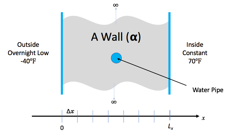
You keep the inside temperature of the house always at 70 degrees F. But, there is an overnight storm coming. The outside temperature is expected to drop to -40 degrees F for 15.5 hours. Will your pipes freeze before the storm is over?
Governing Equations
Heat conduction is governed by the partial differential (PDE)… \[\frac{\partial u}{\partial t} - \nabla \cdot \alpha \nabla u = 0\]
where u is the temperature through the wall at spatial positions, x, and times, t, \( \alpha \), is the thermal diffusivity of the material(s) comprising the wall. This equation is known as the Diffusion Equation and also the Heat Equation.
We make some simplifying assumptions…
- The wall can be treated as homogenous in material.
- In effect, we ignore the fact that part of the wall has a pipe filled with water running through it.
- The thermal diffusivity of the wall material, \( \alpha \) is constant for all space and time.
- The only heat source is from initial and/or boundary conditions.
- We will deal only with the one dimensional problem in Cartesian coordinates.
- That is heat along the dimension through the wall between inside and outside.
- We will discretize with constant spacing in both space, \(\Delta x\) and time, \(\Delta t\).
The PDE simplifies to the one dimensional heat equation… \[\frac{\partial u}{\partial t} = \alpha \frac{\partial^2 u}{\partial x^2}\]
Discretization
Using difference equations as approximations for derivatives, we can discretize, independently, the left- and right-hand sides of equation 2
For the left-hand side, we can approximate the first derivative of u with respect to time, t, by the forward difference equation… \[\frac{\partial u}{\partial t} \Bigr\vert_{t_{k+1}} \approx \frac{u_i^{k+1}-u_i^k}{\Delta t}\]
For the right-hand side, we can approximate the the second derivative of u with respect to space, x, by the centered difference equation… \[\alpha \frac{\partial^2 u}{\partial x^2}\Bigr\vert_{x_i} \approx \alpha \frac{u_{i-1}^k-2u_i^k+u_{i+1}^k}{\Delta x^2}\]
Setting equations 3 and 4 equal to each other and re-arranging terms, we arrive at the following update scheme for producing the temperatures at the next time, k+1, from temperatures at the current time, k, as \[u_i^{k+1} = ru_{i+1}^k+(1-2r)u_i^k+ru_{i-1}^k\]
where \( r=\alpha\frac{\Delta t}{\Delta x^2} \)
Is there anything in this numerical treatment that feels like a mesh? (Click to expand!)
In the process of discretizing the PDE, we have defined a fixed spacing in x and a fixed spacing in t as shown in the figure here

This is essentially a uniform mesh. Later lessons here address more sophisticated discretizations in space and in time which depart from these often inflexible fixed spacings.
Exercise #1: Implement FTCS
% ls
args.C    crankn.C  ftcs.C  heat.C  makefile  tools       utils.C
check.sh  exact.C   Half.H  heat.H  Double.H  upwind15.C
The function, solution_update_ftcs, is defined in ftcs.C without its body.
static bool             // false if unstable, true otherwise
solution_update_ftcs(
    int n,              // # of temperature samples in space
    Double *uk1,        // new temperatures @ t = k+1
    Double const *uk0,  // old/last temperatures @ t = k
    Double alpha,       // thermal diffusivity
    Double dx,          // spacing in space, x
    Double dt,          // spacing in time, t
    Double bc_0,        // boundary condition @ x=0
    Double bc_1         // boundary condition @ x=Lx
)
{
Using eq. 5, implement the body of this function (Click to expand!)
    Double const r = alpha * dt / (dx * dx);

    // Sanity check for stability
    if (r > 0.5) return false;

    // Update the solution using FTCS algorithm
    for (int i = 1; i < n-1; i++)
        uk1[i] = r*uk0[i+1] + (1-2*r)*uk0[i] + r*uk0[i-1];

    // Impose boundary conditions for solution indices 0 & n-1
    uk1[0  ] = bc0;
    uk1[n-1] = bc1;

    return true;
}
Edit ftcs.C and implement the FTCS numerical algorithm by coding the body of this function.
Exercise #2: Build and Test
To compile the code you have just written…
make heat
A note on getting help
% make
without any target specified will display a set of convenient make targets.
Show make output (Click to expand!)
Targets:
    heat: makes the default heat application (double precision)
    heat-half: makes the heat application with half precision
    heat-single: makes the heat application with single precision
    heat-double: makes the heat application with double precision
    heat-long-double: makes the heat application with long-double precision
    PTOOL=[gnuplot,matplotlib,visit] RUNAME=<run-dir-name> plot: plots results
    check: runs various tests confirming steady-state is linear
% ./heat --help
Show help output (Click to expand!)
Usage: ./heat <arg>=<value> <arg>=<value>...
    runame="heat_results"               name to give run and results dir (char*)
    alpha=0.2         material thermal diffusivity (sq-meters/second) (fpnumber)
    lenx=1                                   material length (meters) (fpnumber)
    dx=0.1                x-incriment. Best if lenx/dx==int. (meters) (fpnumber)
    dt=0.004                                    t-incriment (seconds) (fpnumber)
    maxt=2       >0:max sim time (seconds) | <0:min l2 change in soln (fpnumber)
    bc0=0                   boundary condition @ x=0: u(0,t) (Kelvin) (fpnumber)
    bc1=1             boundary condition @ x=lenx: u(lenx,t) (Kelvin) (fpnumber)
    ic="const(1)"               initial condition @ t=0: u(x,0) (Kelvin) (char*)
    alg="ftcs"                            algorithm ftcs|upwind15|crankn (char*)
    savi=0                                   save every i-th solution step (int)
    save=0                              save error in every saved solution (int)
    outi=100                      output progress every i-th solution step (int)
    noout=0                                       disable all file outputs (int)
    prec=2           precision 0=half/1=float/2=double/3=long double (int const)
Examples...
    ./heat dx=0.01 dt=0.0002 alg=ftcs
    ./heat dx=0.1 bc0=273 bc1=273 ic="spikes(273,5,373)"
About the initial condition (ic) argument… (Click to expand!)
The initial condition argument, ic, handles a few interesting cases
- Constant,
ic="const(V)" -
Set initial condition to constant value,
V - Ramp,
ic="ramp(L,R)" -
Set initial condition to a linear ramp having value
L@ x=0 andR@ x=\(L_x\). - Step,
ic="step(L,Mx,R)" -
Set initial condition to a step function having value
Lfor all x<Mx and valueRfor all x>=Mx. - Random,
ic="rand(S,B,A)" -
Set initial condition to random values in the range [B-A,B+A] using seed value
S. - Sin,
ic="sin(Pi*x)" -
Set initial condition to \(sin(\pi x)\).
- Spikes,
ic="spikes(C,A0,X0,A1,X1,...)" -
Set initial condition to a constant value,
Cwith any number of spikes where each spike is the pair,Aispecifying the spike amplitude andXispecifying its position in, x.
Default Run
Run the application with default arguments (e.g. don’t specify any) and see what happens…
Default run output (Click to expand!)
% ./heat
    runame="heat_results"
    prec="double"
    alpha=0.2
    lenx=1
    dx=0.1
    dt=0.004
    maxt=2
    bc0=0
    bc1=1
    ic="const(1)"
    alg="ftcs"
    savi=0
    save=0
    outi=100
    noout=0
Iteration 0000: last change l2=0.0909091
Iteration 0100: last change l2=2.42918e-06
Iteration 0200: last change l2=4.86446e-07
Iteration 0300: last change l2=1.00929e-07
Iteration 0400: last change l2=2.09483e-08
Iteration 0500: last change l2=4.41684e-09
Counts: Adds:24500, Mults:25001, Divs:1005, Bytes:176
Before running, the application dumps its command-line arguments so the user can
see what parameters it was run with. In this case, you are seeing the default
values. It then runs the problem as defined by the command-line arguments and
saves result files, as needed, to the directory specified by the runame= argument.
Understanding the output and results
To list the most recently created entries in the current directory, run the following command…
% ls -1t | head -n 1
heat_results
The entry heat_results is a directory containing some files created by the
application. To determine what kind of files they are, run the following
command…
% file heat_results/*.*
heat_results/clargs.out:                    ASCII text
heat_results/heat_results_soln_00000.curve: ASCII text
heat_results/heat_results_soln_final.curve: ASCII text
For this simple application, the results are uncomplicated. They are ASCII text files containing two columns of data. To see an example, run the command
% cat heat_results/heat_results_soln_final.curve
# Temperature
       0        0
     0.1   0.1039
     0.2   0.2073
     0.3   0.3101
     0.4   0.4119
     0.5   0.5125
     0.6   0.6119
     0.7   0.7101
     0.8   0.8073
     0.9   0.9039
       1        1
The first column is each spatial position, \(x_{i}\) and the second column is the temperature, u, at that spatial position. The name of the file indicates the time of the solution data stored therein.
Testing The heat Application
Before we use our new application to solve our simple science question, how can we assure ourselves that the code we have written is not somehow seriously broken?
Can you think ways to sanity check the our code? (Click to expand!)
- Compare it to known, validated numerical solutions.
- Compare it to known analytical solutions.
- Confirm its behavior at steady state.
In any case, think about how you would measure error.
We know, maybe even intuitively, that if we maintain constant temperatures at \(A @ x=0\) and \(B @ x=L_x\), then after a long time (e.g. when the solution reaches steady state), we expect it to be a simple linear variation between temperatures A and B. For example, observe what happens after a long time in the one dimensional example below.

Construct a suitable command-line to easily confirm a linear steady state (Click to expand!)
Since the default length is 1 and the default boundary conditions are 0 and 1, we just need to run the problem for a long time. But, to be a little more thorough, it is even better to start with a random initial condition too.
% ./heat dx=0.25 maxt=100 ic="rand(125489,100,50)" runame=test
How do you confirm results after a long time are a linear steady state? (Click to expand!)
Examine the initial and final results file and confirm even a random input still yields a final result where \(u=x_{i}\) for all rows of the results file
% cat test/test_soln_00000.curve
# Temperature
       0    69.09
    0.25    143.6
     0.5     96.3
    0.75    52.61
       1    131.6
% cat test/test_soln_final.curve
# Temperature
       0        0
    0.25     0.25
     0.5      0.5
    0.75     0.75
       1        1
Exercise #3: Use Applicaton to Do Some Science
Back to our original problem…will our water pipes freeze?
Additional Information / Assumptions
| Material | Thermal Diffusivity (sq-meters/second) |
| Wood | \(8.2 \times 10^{-8}\) |
| Adobe Brick | \(2.7 \times 10^{-7}\) |
| Common (red) Brick | \(5.2 \times 10^{-7}\) |
- Outside temp has been same as inside temp for a long time, 70 degrees F
- Night/Storm will last 15.5 hours @ -40 degrees F
- Walls are 0.25 meters thick wood and pipe is 0.1 meters in diameter
- Pipe will freeze if center point drops below freezing.
Note: An all too common issue in simulation applications is being sure data is input in the correct units. Take care!
Determine the command-line to run for our simple science problem? (Click to expand!)
./heat runame=wall alpha=8.2e-8 lenx=0.25 dx=0.01 dt=100 outi=100 savi=1000 maxt=55800 bc0=233.15 bc1=294.261 ic="const(294.261)"
Exercise #4: Analyze Results and Do Some Science
Its time to use the results from our simulation to answer the science question of interest. Below we plot results
make plot PTOOL=gnuplot RUNAME=wall
Depending on your situation, the above command may or may not produce a plot looking like below.
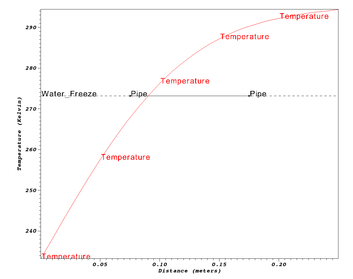
Will the pipes freeze? (Click to expand!)
No.
Challenges with Custom Coding
We all like to write code and build useful tools. However, it is all too easy to see the unfamiliar as an impediment rather than enabler in reaching our sience goals. However, this is a slippery slope. We often start with relatively simple goals and over time wish to evolve our software solutions to ever more challenging science problems.
Examine the lines of code of the complete application here
% wc -l *.[CH]
   125 args.C      # User interface
    94 crankn.C    # Alternative (implicit) solver
    43 exact.C     # Testing support (exact solns for some cases)
    12 ftcs.C      # FTCS (explicit) solver
   222 heat.C      # Main application
    22 heat.H      # Modularization
   115 Double.H    # Performance tracking
    27 upwind15.C  # Alternative (explicit) solver
   157 utils.C     # Utilities, I/O, Data formats
   817 total

  4575 Half.H      # Half precision floats (half.sourceforge.net)
Developing generally useful science applications involves many considerations and software engineering challenges.
- More complex physical phenomena
- Heat sources and radiation
- More complex materials
- Laminated, anisotropic and/or non-linear materials
- More complex geometries
- More spatial dimensions
- Non-cartesian coordinate systems
- Larger objects involving billions of discretization points and requiring scalability in all phases of the solution.
- More generality in execution paradigm
- Distributed memory and multi-threading
- Performance portability and various parallel runtimes
- Interoperability of key components
- Discretizers, solvers, time-integrators, optimizers
- More sophsticated software design and implementation
- Documented, sustainable, maintaiable, portable, efficient, scalable, …
By employing numerical packages, we can leave some of the heavy lifting for others and focus more of our effort on the science and/or the parts of the problem we are most passionate about.
Optional Exercises
For any of these optional exercises, we encourage you to submit a show your work upload of your work for review and feedback. It may take us a few days to respond but we would be happy to follow up.
Short / Quick Follow-on Questions
Will the pipes freeze in a common brick wall of same thickness? (Click to expand!)
Yes.
What is the Optimum thickness of an Adobe Brick Wall? (Click to expand!)
0.3-0.4 meters.
Are the assumptions correct?
A common pitfal in numerical modeling is neglecting to ensure fundamental assumptions still hold. In this exercise, to make the problem tractable and a short lesson, we made a number of simplifying assumptions. If the picture below was a more accurate representation of the situation, the wall is composed more of water (in the pipe) than it is of wall

and our numerical model would fail.
Did this in fact happen in our example, above? (Click to expand!)
Maybe. Certainly the pipe is wider than the original picture suggests.
Determine Optimum Wall Thicknesses
What are the minimum thicknesses of walls of Wood, Adobe and Common brick to prevent the pipes from freezing?
When you are done, go to Intro->Submit A Show Your Work using the hands-on
activity name Optimized Walls and upload evidence of your completed solution.
Compare various precisions
The heat application can be made to run using half, single, double and long double
precision. Try each of these and compare time and space performance as well as quality
of the results. How do the various precisions compare in terms of # of operations, time to
solution, memory used and quality of results?
Compare FTCS, Crank-Nicholson and Upwind15 Algorithms
Crank-Nicolson Discretization
Using the Crank-Nicolson discretization, we arrive at the following discretization of equation 2… \[-ru_{i+1}^{k+1}+(1+2r)u_i^{k+1}-ru_{i-1}^{k+1} = ru_{i+1}^k+(1-2r)u_i^k+ru_{i-1}^k\]
where \[r= \alpha \frac{\Delta t}{2 \Delta x^2}\]
In equation 7, the solution at spatial position i and time k+1 now depends not only on values of u at time k but also on other values of u at time k+1. This means each time we advance the solution in time we must solve a linear system; in other words we must solve for all of the values at time k+1 in one step. This is an example of an implicit method. In this case, the system of equations is tri-diagonal – since each update for u at i only uses u at i-1 , i and i+1 – so it is easier to implement than a general matrix solve but is still more complicated than an explicit update.
The code to implement this method is more involved because it involves
doing a tri-diagonal solve. It is in crankn.C. It involves code that
sets up and LU factors the initial matrix. Then, the LU factored matrix
is used on each solution timestep to solve for the new temperatures.
Run the same problems using each of these algorithms and observe total memory usage and operation counts (printed at the end) and provide your explanations for them and in comparison with the FTCS method.
When you are done, go to Intro->Submit A Show Your Work using the hands-on
activity name Crank-Nicholson and upload evidence of your completed solution.
Use The Application to Solve The Pipeline Problem
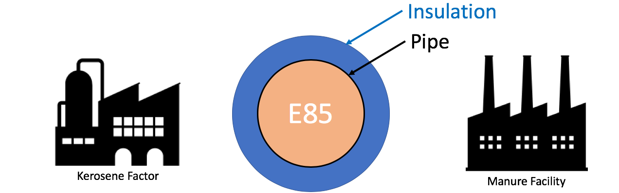
An pipeline carrying Ethenol-85 (E85) runs between a manure processing facility and a kerosene production factory. In the unlikely event that both facilities experience catastrophic explosion (burning methane at the manure facility and burning kerosene at the kerosene facility), that briefly increases the local air temperature on both sides of the pipe to the burning temperature of the respective materials, determine the minimum thermal diffusivity of the material used to coat/insulate the pipe to prevent the E-85 from exploding. Assume the pipe is 36 inches in diameter.
When you are done, go to Intro->Submit A Show Your Work using the hands-on
activity name Pipeline and upload evidence of your completed solution.
Modify the Application to Support Two Materials
Using other research, modify the application to work for a composite wall composed of two materials.
When you are done, go to Intro->Submit A Show Your Work using the hands-on activity
name Composite Wall and upload evidence of your completed solution.