Adjoin time dependent differential equations

Using adjoint for PDE-constrained optimization

At a Glance

Questions	Objectives	Key Points
How can gradients be computed for simulations?	Know PETSc/TAO’s capability for adjoint and optimization	Adjoint enables dynamic constrained optimization
How difficult is it to use the adjoint method?	Understand ingredients needed for adjoint calculation	Jacobian is imperative
	Understand the concern of checkpointing	Performance may depend on checkpointing at large scale

Note: To begin this lesson…

cd HandsOnLessons/adjoint

An Inverse Initial Value Problem

This code demonstrates how to solve an inverse initial value problem for a system of time-dependent PDEs on a 2D rectangular grid. The goal is to determine an optimal initial condition that can minimizes the difference between the simulated result and the reference solution. We will use this example to illustrate the performance considerations for realistic large-scale applications. In particular, we will show how to play with checkpointing and how to profile/tune the performance.

Compile the code

The example ex5opt_ic.c can be compiled with

make ex5opt_ic

To clean the example, do

make clean

ATPESC participants do not need to compile code because binaries are available in the ATPESC project folder on Cooley.

Command line options

You can determine the command line options available for this particular example by doing

./ex5opt_ic -help

and show the options related to TAO only by doing

./ex5opt_ic -help | grep tao

Problem being solved

The underlying PDE models reaction and diffusion of two chemical species that can produce a variety of patterns. It is widely used to describe pattern-formation phenomena in biological, chemical and physical systems. The concentrations of the two species are calculated according to the equation \[\frac{d\mathbf{u}}{dt} = D_1 \nabla^2 \mathbf{u} - \mathbf{u} \mathbf{v}^2 + \gamma(1 -\mathbf{u}) \\ \frac{d\mathbf{v}}{dt} = D_2 \nabla^2 \mathbf{v} + \mathbf{u} \mathbf{v}^2 - (\gamma + \kappa)\mathbf{v}\]

The spatial pattern for the time interval [0,200] seconds is shown in the following figure.

Figure 1

Given the pattern (observation) at the final time of the simulation, we want to determine the initial pattern that can minimize the difference between the simulated result and the observation. \[\text{minimize}_{X_0} \| X - X^{ref}\|\]

Run 1: Monitor solution graphically

mpiexec -n 4 ./ex5opt_ic -forwardonly -ts_type rk -ts_rk_type 3 -ts_max_steps 20 -ts_monitor -ts_monitor_draw_solution

-forwardonly perform the forward simulation without doing optimization
-ts_type rk -ts_rk_type 3 changes the time stepping algorithm to a 3rd-order Runge-Kutta method
-ts_monitor_draw_solution monitors the progress for the solution at each time step
Add -draw_pause -2 if you want to pause at the end of simulation to see the plot

Run 2: Optimal checkpointing schedule

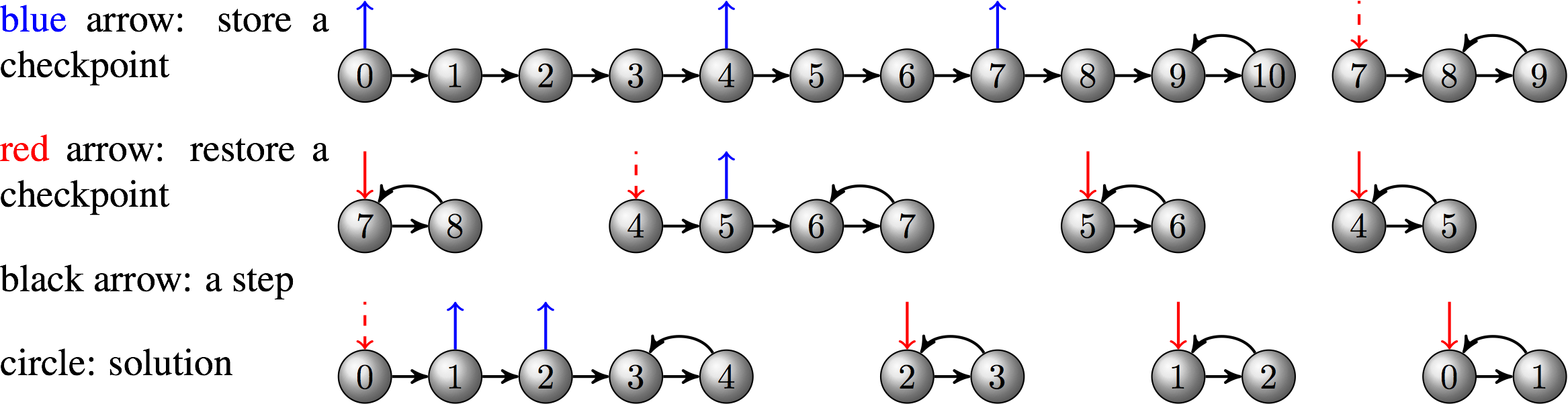
By default, the checkpoints are stored in binary files on disk. Of course, this may not be a good choice for large-scale applications running on high-performance machines where I/O cost is significant. We can make the solver use RAM for checkpointing and specify the maximum allowable checkpoints so that an optimal adjoint checkpointing schedule that minimizes the number of recomputations will be generated.

mpiexec -n 4 ./ex5opt_ic -ts_type rk -ts_rk_type 3 -ts_adapt_type none \
                     -ts_max_steps 10 -ts_monitor -ts_adjoint_monitor \
                     -ts_trajectory_type memory -ts_trajectory_max_cps_ram 3 \
                     -ts_trajectory_monitor -ts_trajectory_view -tao_max_it 1

-tao_max_it 1 forces the optimization to stop after one iteration so that we can focus on the output related to the adjoint checkpointing. The output corresponds to the schedule depicted by the following diagram:

Questions

What will happen if we add the option -ts_trajectory_max_cps_disk 2 to specify there are two available slots for disk checkpoints?

Looking at the output, we will find that the new schedule uses both RAM and disk for checkpointing and takes two less recomputations.

Run 3: Monitor the optimization progress

mpiexec -n 4 ./ex5opt_ic -ts_type rk -ts_rk_type 3 -ts_adapt_type none -ts_max_steps 5 -ts_trajectory_type memory -ts_trajectory_solution_only 0 -tao_monitor -tao_view
  0 TAO,  Function value: 8.48202,  Residual: 7.02449
  1 TAO,  Function value: 1.72589,  Residual: 2.46827
  2 TAO,  Function value: 0.556599,  Residual: 1.75419
  3 TAO,  Function value: 0.181113,  Residual: 0.698038
  4 TAO,  Function value: 0.0919628,  Residual: 0.390951
  5 TAO,  Function value: 0.0330733,  Residual: 0.276822
  6 TAO,  Function value: 0.0137442,  Residual: 0.205942
  7 TAO,  Function value: 0.0032463,  Residual: 0.0925536
  8 TAO,  Function value: 0.000876358,  Residual: 0.0469696
  9 TAO,  Function value: 0.000172022,  Residual: 0.0205954
 10 TAO,  Function value: 2.32065e-05,  Residual: 0.00808249
 11 TAO,  Function value: 1.00524e-05,  Residual: 0.00695292
 12 TAO,  Function value: 2.19094e-06,  Residual: 0.00192488
 13 TAO,  Function value: 9.37506e-07,  Residual: 0.00115926
 14 TAO,  Function value: 2.79883e-07,  Residual: 0.000907609
 15 TAO,  Function value: 7.22e-08,  Residual: 0.000346602
 16 TAO,  Function value: 3.51499e-08,  Residual: 0.000184429
 17 TAO,  Function value: 1.48741e-08,  Residual: 0.000117587
 18 TAO,  Function value: 7.83221e-09,  Residual: 9.19265e-05
 19 TAO,  Function value: 2.14226e-09,  Residual: 4.54118e-05
 20 TAO,  Function value: 8.99022e-10,  Residual: 2.91421e-05
 21 TAO,  Function value: 3.28239e-10,  Residual: 2.06652e-05
 22 TAO,  Function value: 1.85795e-10,  Residual: 2.71364e-05
 23 TAO,  Function value: 1.14498e-10,  Residual: 2.32933e-05
 24 TAO,  Function value: 8.12369e-11,  Residual: 2.22391e-05
 25 TAO,  Function value: 1.87747e-11,  Residual: 7.85018e-06
 26 TAO,  Function value: 7.29614e-12,  Residual: 5.02828e-06
 27 TAO,  Function value: 1.72522e-12,  Residual: 1.07136e-06
 28 TAO,  Function value: 1.0259e-12,  Residual: 7.63383e-07
 29 TAO,  Function value: 1.72785e-13,  Residual: 3.91911e-07
 30 TAO,  Function value: 1.0509e-13,  Residual: 2.75909e-07
 31 TAO,  Function value: 4.02491e-14,  Residual: 1.7222e-07
 32 TAO,  Function value: 1.5385e-14,  Residual: 1.21345e-07
 33 TAO,  Function value: 3.20145e-15,  Residual: 7.81137e-08
 34 TAO,  Function value: 1.66953e-15,  Residual: 5.25802e-08
 35 TAO,  Function value: 3.39432e-16,  Residual: 3.16327e-08
 36 TAO,  Function value: 9.68078e-17,  Residual: 1.15783e-08
 37 TAO,  Function value: 8.23443e-17,  Residual: 1.68247e-08
 38 TAO,  Function value: 1.53356e-17,  Residual: 7.63537e-09
Tao Object: 4 MPI processes
  type: blmvm
  Gradient steps: 0
  Mat Object: (tao_blmvm_) 4 MPI processes
    type: lmvmbfgs
    rows=8192, cols=8192
      Scale type: diagonal
      Scale history: 1
      Scale params: alpha=1., beta=0.5, rho=1.
      Convex factors: phi=0., theta=0.125
      Max. storage: 5
      Used storage: 5
      Number of updates: 37
      Number of rejects: 0
      Number of resets: 1
  TaoLineSearch Object: 4 MPI processes
    type: more-thuente
    maximum function evaluations=30
    tolerances: ftol=0.0001, rtol=1e-10, gtol=0.9
    total number of function evaluations=0
    total number of gradient evaluations=0
    total number of function/gradient evaluations=1
    using variable bounds
    Termination reason: 1
  Active Set subset type: subvec
  convergence tolerances: gatol=1e-08,   steptol=0.,   gttol=0.
  Residual in Function/Gradient:=7.63537e-09
  Objective value=1.53356e-17
  total number of iterations=38,                          (max: 2000)
  total number of function/gradient evaluations=41,      (max: 4000)
  Solution converged:    ||g(X)|| <= gatol

-tao_draw_solution can visualize the solution at each optimization iteration

Questions

Examine the source code and find the user-provided functions for TAO, TS, and TSAdjoint respectively.

Essential functions we have provided are FormFunctionGradient for TAO, TSIFunction and TSIJacobian for TS, RHSJacobianP for TSAdjoint. Because of the integral in the objective function, extra functions including CostIntegrand, DRDYFunction and DRDPFunction are given to TSAdjoint.

Run 4: Implicit time integration method

Now we switch to an implicit method (Crank-Nicolson) using fixed stepsize, which is the default setting in the code. At each time step, a nonlinear system is solved by the PETSc nonlinear solver SNES.

mpiexec -n 12 ./ex5opt_ic -ts_max_steps 5 -log_view -tao_monitor

-snes_monitor can show the progress of SNES
-ts_monitor can show the progress of TS
-log_view prints a summary of the logging

A snippet of the summary:

...
Phase summary info:
   Count: number of times phase was executed
   Time and Flop: Max - maximum over all processors
                   Ratio - ratio of maximum to minimum over all processors
   Mess: number of messages sent
   Avg. len: average message length (bytes)
   Reduct: number of global reductions
   Global: entire computation
   Stage: stages of a computation. Set stages with PetscLogStagePush() and PetscLogStagePop().
      %T - percent time in this phase         %F - percent flop in this phase
      %M - percent messages in this phase     %L - percent message lengths in this phase
      %R - percent reductions in this phase
   Total Mflop/s: 10e-6 * (sum of flop over all processors)/(max time over all processors)
------------------------------------------------------------------------------------------------------------------------
Event                Count      Time (sec)     Flop                             --- Global ---  --- Stage ---   Total
                   Max Ratio  Max     Ratio   Max  Ratio  Mess   Avg len Reduct  %T %F %M %L %R  %T %F %M %L %R Mflop/s
------------------------------------------------------------------------------------------------------------------------

--- Event Stage 0: Main Stage

VecDot              1130 1.0 3.9795e-01 1.4 1.59e+06 1.0 0.0e+00 0.0e+00 1.1e+03  4  1  0  0  8   4  1  0  0  8    46
VecMDot             1919 1.0 5.9272e-01 2.0 5.40e+06 1.0 0.0e+00 0.0e+00 1.9e+03  5  4  0  0 14   5  4  0  0 14   106
VecNorm             3678 1.0 8.1644e-01 1.3 5.18e+06 1.0 0.0e+00 0.0e+00 3.7e+03  9  4  0  0 27   9  4  0  0 27    74
...

Questions

Where is the majority of CPU time spent?

Of course answer may vary depending on the settings such as number of procs, problem size, and solver options. Typically most of the time should be spent on VecMDot or MatMult

How can we improve performance?

Use memory instead of disk for checkpointing(-ts_trajectory_type memory -ts_trajectory_solution_only 0); 2. Tune the time stepping solver, nonlinear solver, linear solver, preconditioner and so forth.

Run 5: Scale up the problem

We use explicit Runge-Kutta methods for time integration, and increase the grid resolution to 512 X 512.

mpiexec -n 12 ./ex5opt_ic -ts_type rk -ts_rk_type 3 -ts_adapt_type none -ts_max_steps 5 -ts_trajectory_type memory -ts_trajectory_solution_only 0 -tao_monitor -da_grid_x 512 -da_grid_y 512

Questions

Does the optimization converge? If not, can you fix it?

No. The PDE solution blows up. As we decrease the grid spacing, the stepsize should be reduced according to CFL condition. For example, adding -ts_dt 0.1 should work.

Further information

Because this example uses DMDA, Jacobian can be efficiently approximated using finite difference with coloring. You can use the option -snes_fd_color to enable this feature.

Out-Brief

We have used PETSc to demonstrate the adjoint capability as an enabling technology for dynamic-constrained optimization. In particular, we investigated an inverse initial value porblem built on a time-dependent reaction-diffusion PDE.

We have shown the basic usage of the adjoint solver as well as functionalities that can facilitate rapid development, diagnosis and performance profiling.

At a Glance

An Inverse Initial Value Problem

Compile the code

Command line options

Problem being solved

Run 1: Monitor solution graphically

Run 2: Optimal checkpointing schedule

Questions

Run 3: Monitor the optimization progress

Questions

Run 4: Implicit time integration method

Questions

Run 5: Scale up the problem

Questions

Further information

Out-Brief

Further Reading