Conformal Unstructured Mesh Adaptation for Linear Elastic Tensial Loading

Adaptive MFEM+PUMI Workflow

MFEM with PUMI Conformal Unstructured Mesh Adaptation

At A Glance

Questions	Objectives	Key Points
How can I define a simulation on a complex geometric model?	Demonstrate model defeaturing and mesh generation pre-processing tools	Complex models require robust pre-processing tools!
	Demonstrate the power of geometric model classification	Automated simulation tools designed for scientists and engineers working with real CAD models problem definition information must be specified on the geometric model - not the mesh.
How can I reliably and efficiently execute simulations?	Demonstrate an adaptive MFEM+PUMI elastic analysis	Adaptation is critical to automated, robust, and efficient simulation of simulations with transient behavior in which a static mesh defined a-priori will fail.

Before you begin, first Open the Answers Form in a separate browser tab/window. We will be entering responses to questions here that are placed throughout the lesson.

The MFEM+PUMI examples are prepared for execution on Cooley at ALCF. Except where noted, all commands shown below should be executed in a terminal logged into Cooley. In each new terminal first prepare your environment by running the commands listed in the following section.

Note, each step can be performed independently; we encourage you to go through them in order though. If there are issues running the examples, or you wish to skip ahead you will find the execution output in the expectedOutput directory.

To begin this lesson

Copy the example directory to your home directory

rsync -aP /projects/ATPESC2018/FASTMath/HandsOnLessons/mfem-pumi-lesson ~/.

Enter the lesson directory
```
cd ~/mfem-pumi-lesson
```
Setup your environment (ensures that your environment is using the @default + +mvapich2-2.3rc1 dotkit pacakges)
```
source setup.sh
```

Geometric Model Defeaturing

Geometric models are often provided by design engineers and include many features that are not required for simulation. The left side of Figure 1 depicts the geometric model of a Tokamak fusion reactor that has multiple bolts, nuts, and brackets that have no influence on the frequency analysis. These features are removed from the Parasolid CAD model by the Simmetrix SimModSuite tools by calling Parasolid kernel APIs to delete the faces and ‘heal’ the remaining hole via extensions of the bounding edges and faces. The right side of Figure 1 depicts the defeatured Tokamak model. In a model with this level of complexity that engineers and scientists running the simulation often must coordinate to create the `as-simulated’ model.

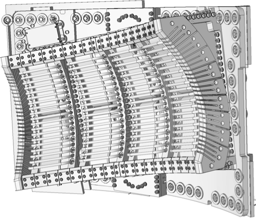
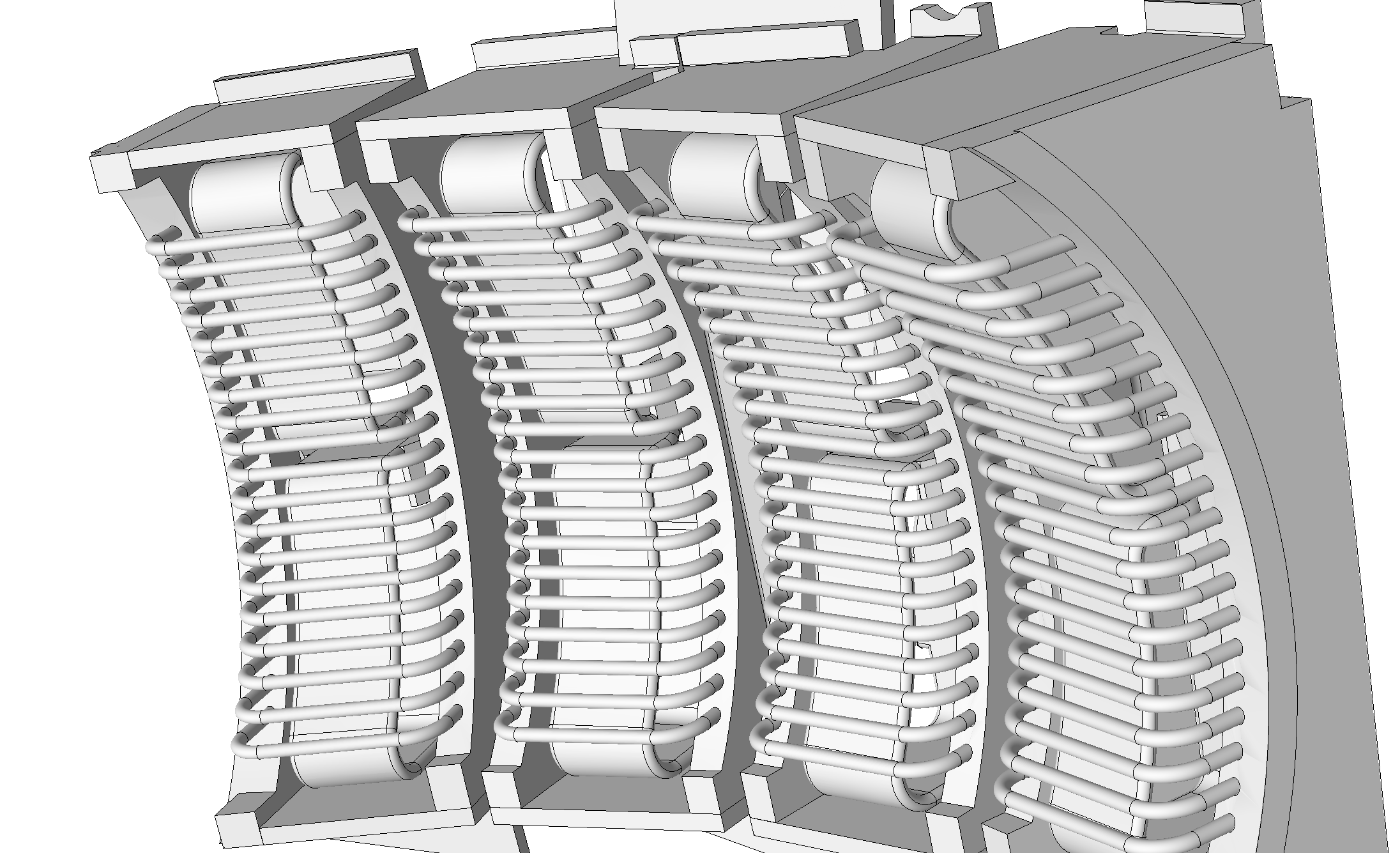
Figure 1. Initial (left) and defeatured (right) Tokamak antenna geometric model

For this hands-on we removed a few small faces on the RPI Formula Hybrid suspension upright shown in Figure 2 to illustrate a few key characteristics of the mesh generation procedures.

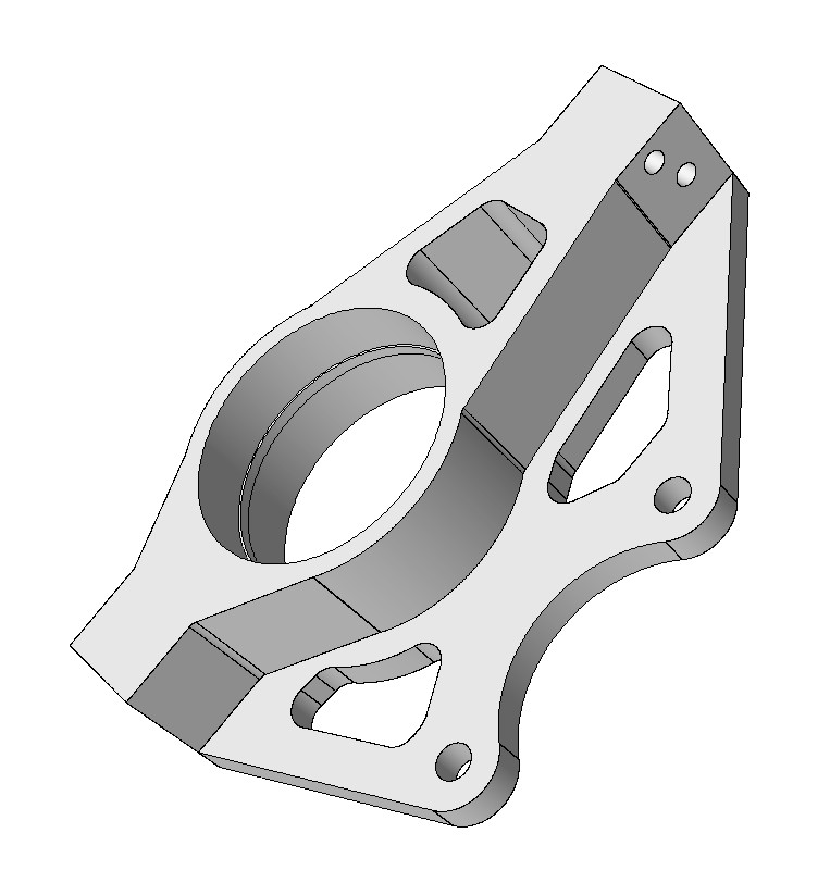
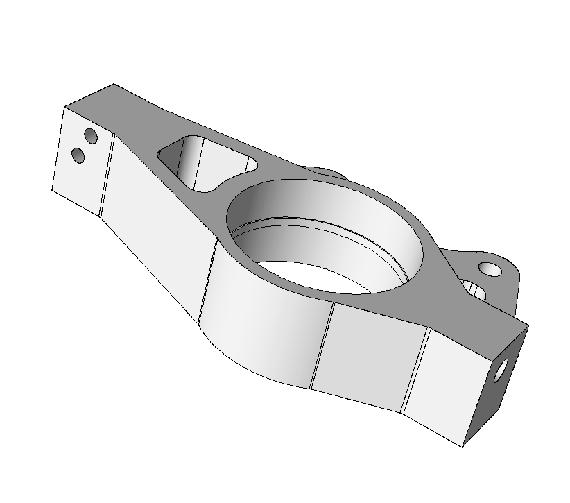
Figure 2. RPI Formula Hybrid suspension upright

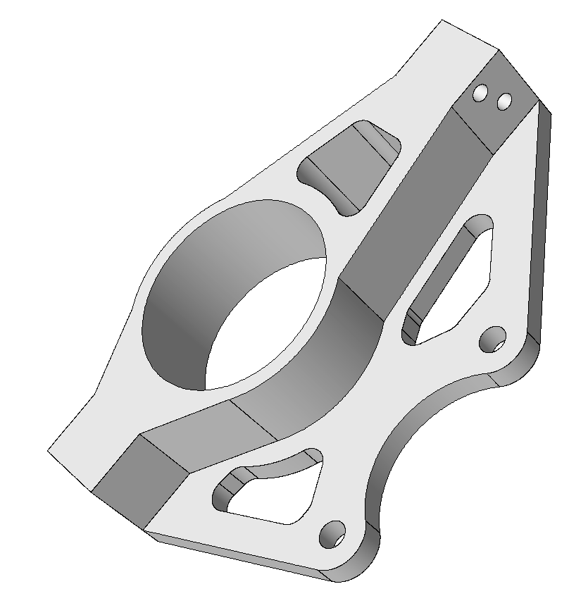
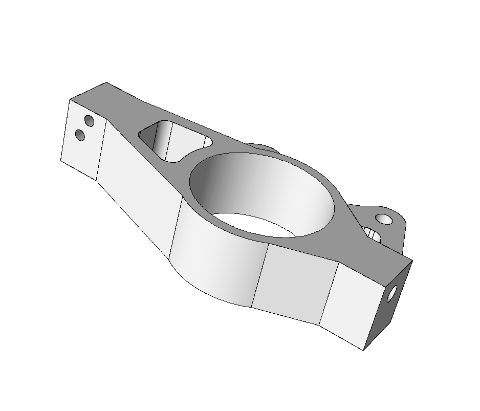
Figure 3. RPI Formula Hybrid suspension upright with small faces removed

In the Mesh Generation step we will generate and compare meshes of the initial and defeatured geometric models.

Optional - Run SimModeler to defeature the upright.

Launch the VNC

The Setup page has more detailed, and scripted, instructions to launch the VNC.

Run SimModeler:

cd ~/mfem-pumi-lesson/SimModeler6.0-180525/
./simmodeler

Remove a small face

click ‘File->Import Geometry’ and select the upright.x_t model
click the ‘Modeling’ tab
click a small geometric model face
click ‘Delete Faces and Heal’ then click ‘Apply’ to remove the face

Try removing the ring inside the hub by selecting all three of its faces, clicking the ‘+’ symbol to add them to the list, then clicking ‘Apply’.

Problem Definition Introduction

The boundary conditions, initial conditions, material parameters, etc. are specified on the geometric model - not the mesh. In the Problem Definition Section we will describe the mechanism that supports this and the specific boundary conditions for this problem.

Mesh Generation

Now that we have prepared the model and defined the boundary conditions we can proceed with mesh generation using the Simmetrix SimModSuite library APIs. The mesh generation procedures are driven by size controls defined by the user on geometric model entities or defined within geometric primitives that intersect the model (e.g., cubes, spheres, cylinders, etc.). In this example we generate a coarse mesh using a single relative size control applied to the entire model. This control guides the generation procedures to create edges whose lengths are proportional, using our prescribed value, to the length of local geometric model features.

The mesh generator is automated, which in the domain of mesh generation means that it will always produce a valid mesh while doing its best to respect the user specified controls. Note, the features of the geometric model highly dictate what mesh sizes are possible. Specifically:

the mesh topology must exactly respect the geometric model topology, i.e., each geometric model edge has a set of meshes edges classified on it that cover the entire model edge.
in the case of problems on curved domains, the geometry of the typical interpolating point mesh (even using higher-order curved elements) is only an approximation to the original geometric model.

Once the mesh is generated we convert it, in-memory (i.e., using PUMI and SimModSuite APIs), to a PUMI mesh and then write the PUMI mesh to file.

 1) Given the same mesh size controls (e.g., the length of mesh edges),
    the mesh on the initial geometry will:
    a) ... have *more* elements than the mesh of the defeatured geometric model.
    b) ... have *less* elements than the mesh of the defeatured geometric model.
    c) ... have the same number of elements as the mesh of the defeatured geometric model.

qsub -I -n 1 -t 30 -A ATPESC2018 -q training
cd ~/mfem-pumi-lesson/meshGeneration
# generate the mesh on the initial geometric model and create paraview vtu files
./generate --native-model=upright.x_t upright.smd 5kg1
./render upright.x_t 5kg1/ 5kg1_initial_vtu
# generate the mesh on the defeatured model and create paraview vtu files
./generate upright_defeatured_geomsim.smd 5kg1
./render upright_defeatured_geomsim.smd 5kg1/ 5kg1_defeatured_vtu

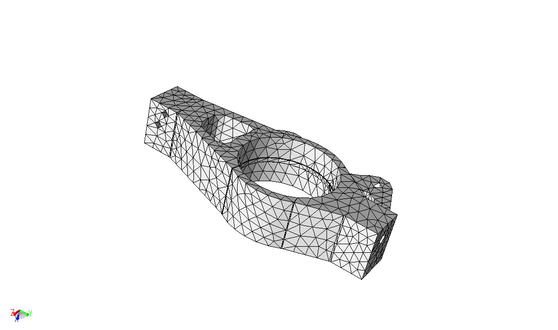
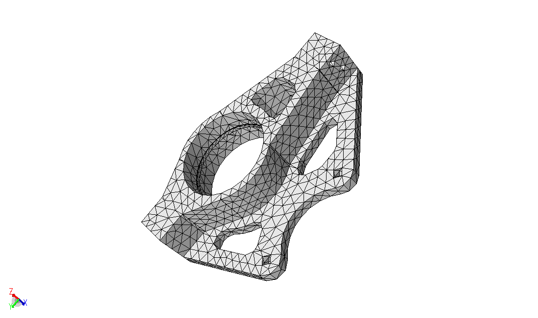
Figure 4. Mesh of initial upright model

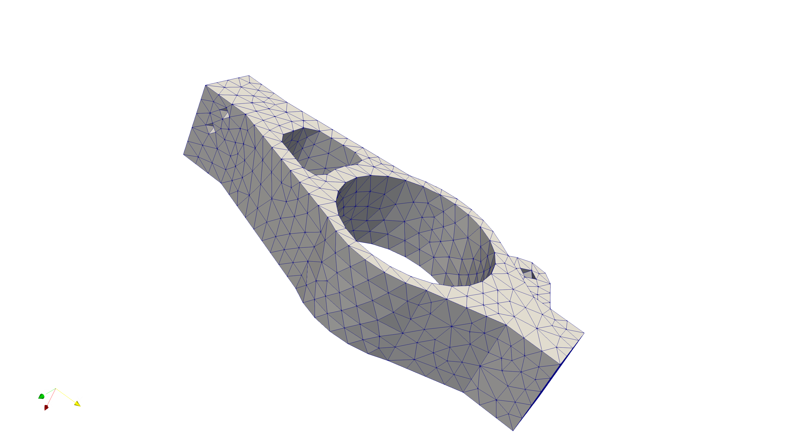
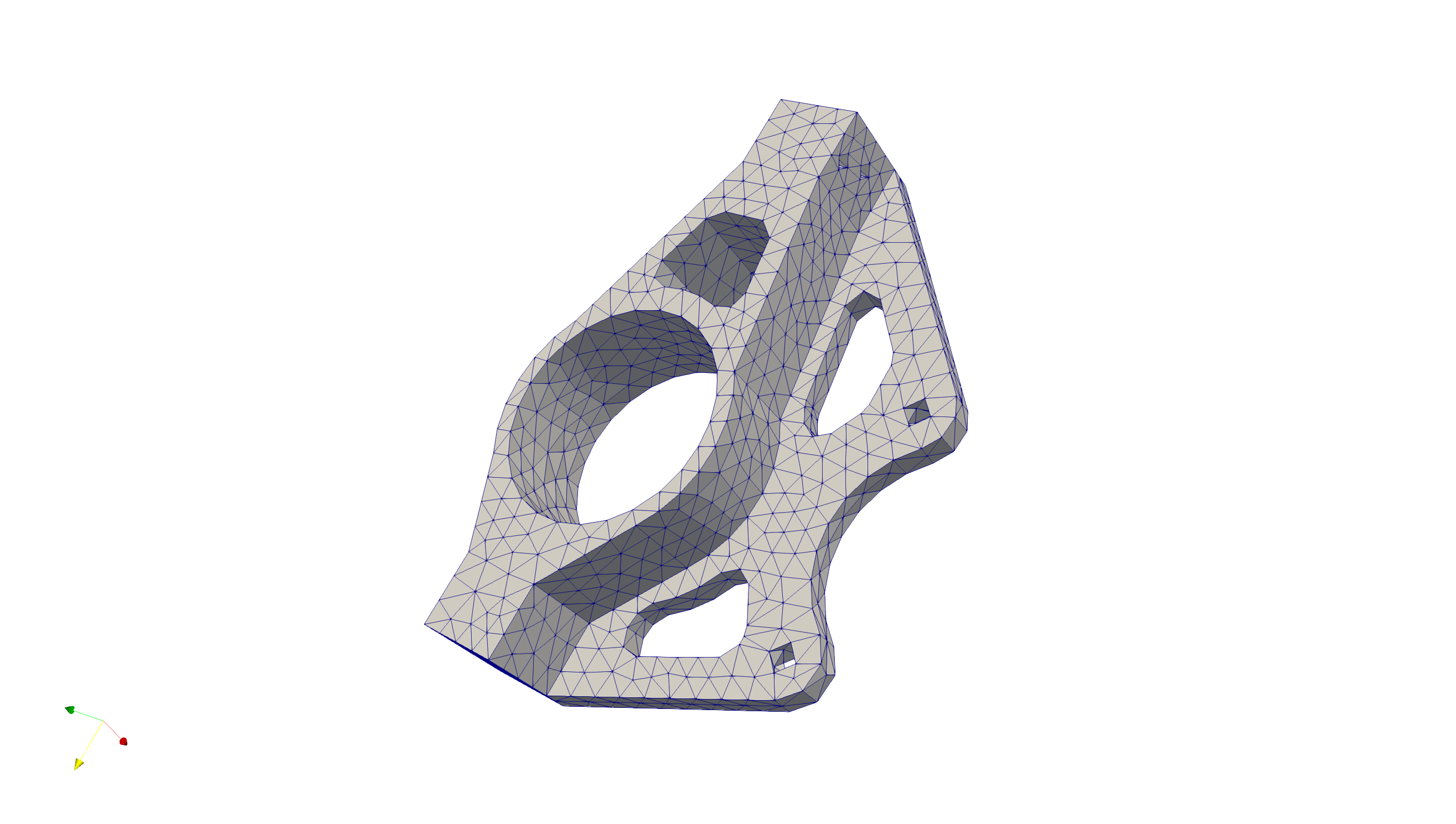
Figure 5. Mesh of defeatured upright model

Optional - Visualize the Initial Meshes

Download the .*vtu files from Here, or use a file transfer utility (e.g., scp, rsync, putty, etc.) to copy the ones you generated to your local machine.

This concludes the day time hands-on. In the evening you’ll have an opportunity to repeat these steps and follow two additional steps before running the adaptive analysis.

Partitioning

Efficient parallel execution requires equally distributing the units of work among the processing resources while keeping communication costs low. The multi-level graph and recursive sectioning geometric methods are among the most commonly available and used methods for partitioning unstructured meshes. In this lesson we will exercise the multi-level graph partitioner (referred to as ‘graph’ below) provided by the Zoltan interface and implemented by ParMETIS. We will then run recursive coordinate bisection (‘RCB’) and recursive inertial bisection (‘RIB’) to produce meshes of with the same part count (number of sub-domains), and compare the results. All three partitioners are targeting an imbalance of 5%; defined as the max element count on any part divided by the average element count across all parts.

qsub -I -n 1 -t 30 -A ATPESC2018 -q training
cd ~/mfem-pumi-lesson/partition
runParma=0
isLocal=0
render=1
mdl=upright_defeatured_geomsim.smd
mesh=5kg1_defeatured/
mpirun -np 4 ./ptnParma $mdl $mesh 5kg1_p4_parmetis/ 4 pmetis kway $isLocal $runParma $render &> graph.out
mpirun -np 4 ./ptnParma $mdl $mesh 5kg1_p4_rcb/ 4 rcb ptn $isLocal $runParma $render &> rcb.out
mpirun -np 4 ./ptnParma $mdl $mesh 5kg1_p4_rib/ 4 rib ptn $isLocal $runParma $render &> rib.out

The entity imbalance information is listed on the lines containing entity imbalance <v e f r>:. The grep command to extract these lines from the outputs is:

       grep 'afterSplit entity imbalance' *.out

The imbalance values follow the definition given above (max count/avg count); i.e., 5% imbalance will be listed as 1.05.

The number mesh entities that are shared with other processes is indirectly indicated on the lines containing weighted TYPE <tot max min avg> where TYPE is vtx, edge, or face. The grep command to extract these lines from the outputs is:

grep 'afterSplit weighted vtx' *.out

If the total (tot) or average (avg) number of entities of a given TYPE is larger relative to another partition then that partition has more replicated entities.

Given the values of the imbalance and shared entity count for each partition (graph, RCB, RIB) above and the content of the [graph|rcb|rib].out files,

2) Which partition has the highest vertex imbalance?
   a)RCB
   b)RIB
   c)multi-level graph

3) Which partition has the most mesh vertices?
   a)RCB
   b)RIB
   c)multi-level graph

 4) Which partition has the highest element imbalance?
    a)RCB
    b)RIB
    c)multi-level graph

The partitioning decisions of RIB and RCB are based on the centroid of mesh elements while the multi-level graph partitioner is using mesh adjacency information (graph vertex = mesh element, graph edge = mesh face shared by two mesh elements).

 5) What causes the boundaries of the RIB and RCB partitions to look jagged
    relative to the multi-level graph partition boundaries?
    a) the placement of the cutting plane versus the coordinates of
    the mesh elements
    b) the intersection of the cutting planes used by the recursive
    sectioning procedures form angular multi-part junctions whereas the multi-level
    graph procedures produce more rounded parts and thus smoother junctions
    c) the multi-level graph procedure uses mesh adjacency information to reduce the
    number of mesh faces on the partition boundaries

All of the above.

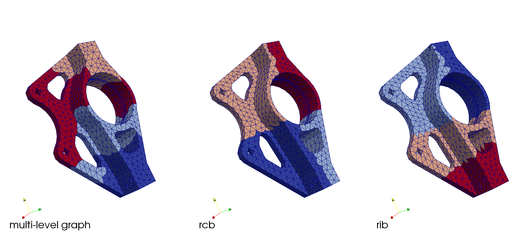
Figure 6. Partitions created with multi-level graph (left), RCB (middle), and RIB (right)

Optional - Visualize the Partitioned Meshes

Download the .*vtu files from Here, or use a file transfer utility (e.g., scp, rsync, putty, etc.) to copy the ones you generated to your local machine.

Problem Definition

We will define a tensile loading on the upright by applying a uniform force on one end (min Y face) and fixing the displacements on the other end (max Y face); as depicted in Figure 7. All other geometric model faces will be unconstrained. No body forces are applied.

Figure 7. Boundary conditions

Using geometric classification of the mesh we can define the boundary conditions on the geometric model without having any knowledge/consideration of the mesh. Geometric classification defines the equal, or greater, order association of mesh entities to geometric model entities. Specifically, a mesh region can only be classified on a geometric model region, a mesh face on a geometric face or region, and so on. Geometric classification is used throughout the set of unstructured mesh tools. For example, in mesh adaptation, classification (along with knowledge of the geometries parametric shape information) is critical for improving the meshes approximation to the geometric model when moving, adding, or removing mesh entities. Further reading on the use of classification is available in Beall et al. 1999 and Ibanez 2016.

A very simple text based interface was defined for this demonstration example to define the two boundary conditions. To specify the geometric model faces with the load applied we add one line with Load followed by another line with the number of faces with that load applied. The geometric model face ids, one per line, are then listed. Using the same convention we define the fixed faces using the string Dirichlet, the number of listed faces, then the list of face ids. The boundary condition specification for this example is listed below. Using the geometric model classification mechanism supports creation of more feature-rich interfaces (command line, file, GUI).

$ cat upright.def
Dirichlet
1
43

Load
1
344

6) Which of the following statements are true? Specifying boundary
   conditions on the geometric allows users to:
   a)... change the mesh without having to modify the boundary condition definition
   b)... specify boundary conditions that vary over the geometric model entity
   c)... automate mesh creation and analysis execution

All of the above.

Adaptive Simulation

This problem solves a linear elasticity model on a cantilever beam. Specifically, we approximate the weak form of \[-div(\sigma(u))=0\]

where \[\sigma(u)=\lambda*div(u)*I+\mu*(\nabla*u+u*\nabla)\]

is the stress tensor corresponding to displacement field \(u\), and \(\lambda=1\) and \(\mu=1\) are the material Lame constants.

Figure 7 depicts the applied boundary conditions; a fixed displacement \(u=0\) on the max Y face and pull force \(f=1.0e-2\) on the min Z face. The specification of these boundary conditions using geometric model entity ids is described in the Problem Definition section.

To control the error without a-priori knowledge of solution we will run this example using mesh adaptation. The adaptive cycle:

solves the problem on an initial uniform coarse mesh,
estimates the discretization error,
defines an isotropic size field from the error estimate,
adapts the mesh using the size field, and
solves the problem on the adapted mesh.

Multiple methods are available for error estimation (see the Further Reading section) and the subsequent size field computation. In this example a patch recovery approach is used.

Given the structure of the geometric model and the specified boundary conditions, we expect that the upper portion (positive Z) of the main hub experiences higher stresses as the lower part is much stiffer. Given this intuition we would expect higher error there and therefore a finer mesh is expected as the result of the meshAdapt.

Run the adaptive simulation:

cd ~/mfem-pumi-lesson/analysis
mpirun -np 2 ./pumi_upright_ex2p -p upright_defeatured_geomsim.smd -bf upright.def -m 2p5kg1/

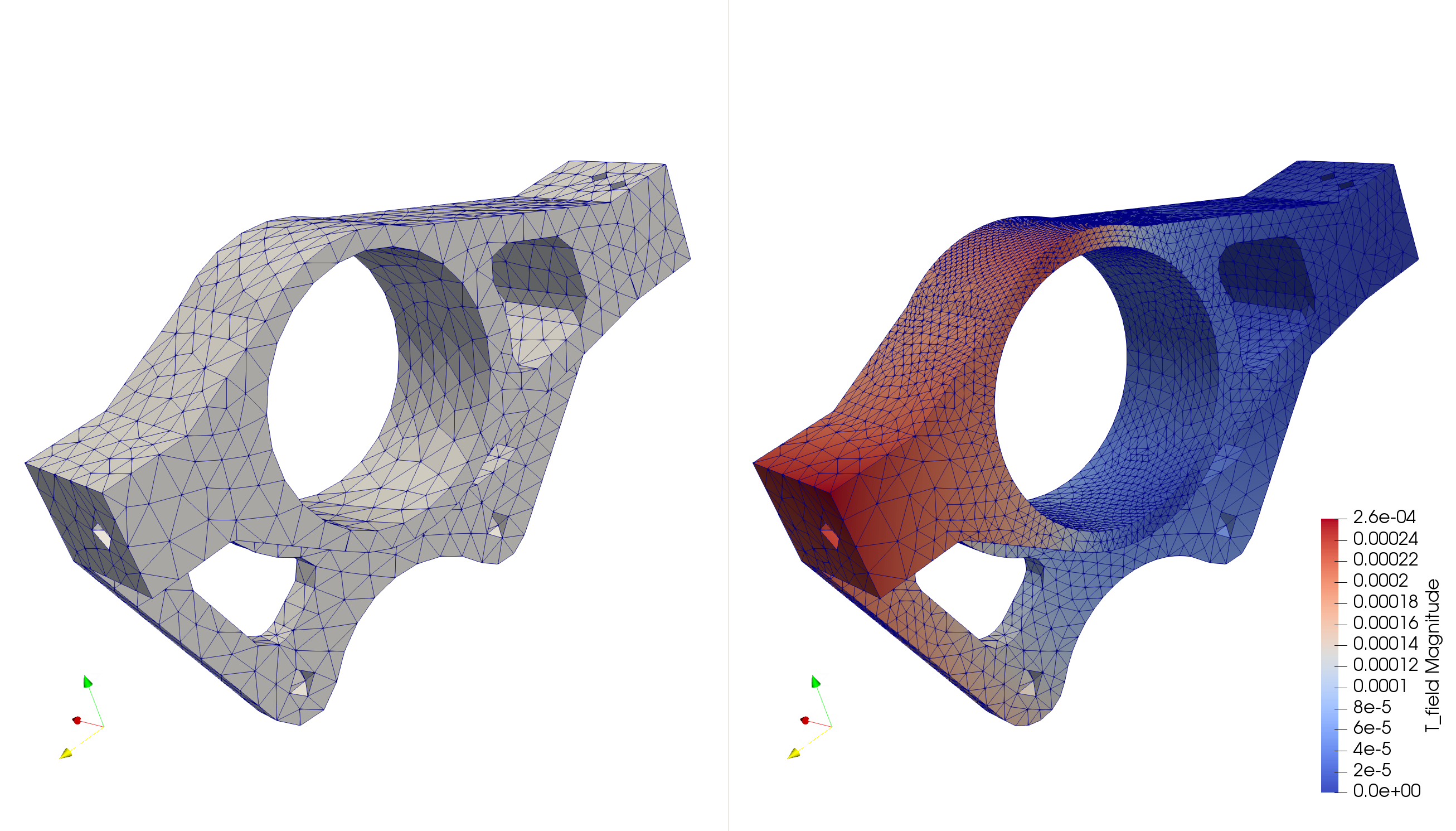
*Figure 8. Initial mesh (left) and final mesh with displacement field (right).

The requested isotropic (same in all directions) edge length is specified with a scalar value at each mesh vertex. In Section 2.1 of Li et al. edge lengths that vary with direction, anisotropic, are specified.

7) How do applications request anisotropic edge lengths from mesh adaptation procedures?

Using a mesh metric tensor that can be decomposed into eigen values and eigen vectors that specify the length of the edges in the principle directions.

Optional - Visualize the analysis results

Download the .*vtu files from Here, or use a file transfer utility (e.g., scp, rsync, putty, etc.) to copy the ones you generated to your local machine.

Get Credit / Points

Be sure to submit a Show Your Work using the hands-on activity name, PUMI_Partitioning or PUMI_Adaptive_Simulation.

Out-Brief

We have exercised a workflow using PUMI and MFEM software components that is based on a high level definition of the problem domain; the geometric model. The PUMI and MFEM software components exchange information on the geometric model, the mesh, and fields on the mesh to provide a robust and extensible set of functionalities that support the needs of multiple applications.